Chapter III: Why does the slanted viewing angle at high latitudes matter?
3. Why does the slanted viewing angle at high latitudes matter?
Optical path refers to the path that light or other electromagnetic radiation takes as it travels from the Earth's surface to a satellite sensor. At high latitudes, this path is longer and more slanted due to the curvature of the Earth and the position of geostationary satellites over the equator (Figure 6). As a result, the signal passes through a thicker layer of the atmosphere, leading to increased attenuation of the signal due to absorption and scattering. Moreover, the longer optical path increases the likelihood of encountering semi-transparent clouds, aerosols, and other atmospheric particles that can distort the signal, leading to difficulties in interpreting the data for critical parameters such as cloud top temperature. This chapter discusses the main phenomena and challenges associated with longer optical paths at high latitudes.
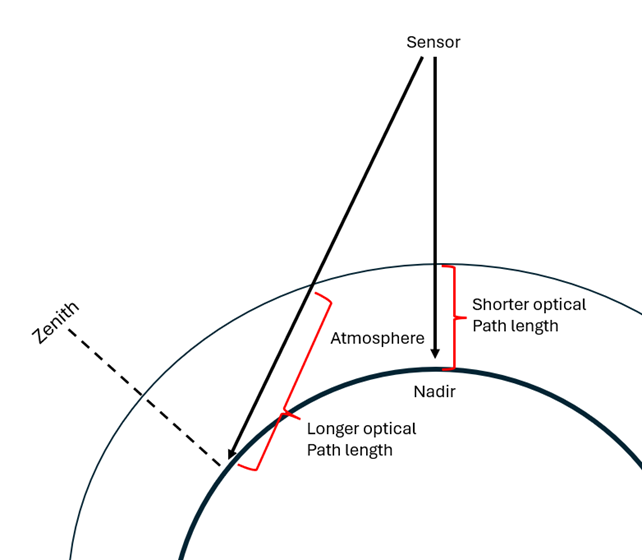
Figure 6: Illustration of the optical path from a GEO-satellite sensor.
2.1 The Role of Parallax Shift in Satellite Image Interpretation
Parallax is the visual phenomenon whereby the position of an object in relation to a background appears to change depending on the viewer's position. Parallax shift can be easily demonstrated with a simple everyday exercise using your thumb and your eyes (Figure 7):
- Hold up your thumb at arm's length in front of you.
- Close your left eye and observe your thumb with your right eye.
- Now, switch eyes - close your right eye and open your left eye.
- Do this a couple of times and note how your thumb seems to shift position against the background. Even though your thumb hasn't moved, it looks like it has jumped sideways.
This phenomenon occurs due to the eyes being in slightly different viewing locations, causing a nearby object, your thumb, to appear to shift relative to the background. As well as in your everyday life, parallax shift is relevant in various fields, including meteorology. This chapter discusses its importance in satellite meteorology and why every forecaster should be aware of it.
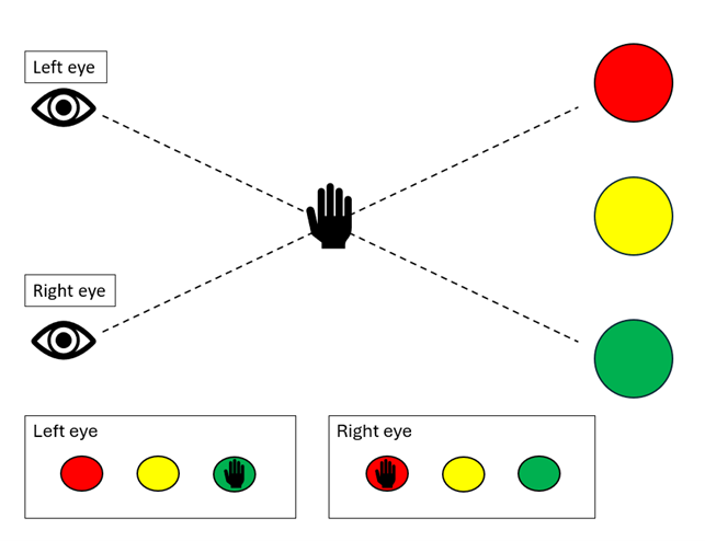
Figure 7: Simple example of parallax shift in everyday life.
In satellite meteorology, the parallax shift phenomenon occurs when the viewing angle of a satellite deviates from the sub-satellite point, also known as the nadir (Figure 8). This results in an object situated between the satellite and the Earth's surface appearing in an erroneous position in the satellite imagery, so that a meteorologist could produce an inaccurate analysis if relying solely on satellite images. It is therefore vital to understand and acknowledge parallax shift for accurate weather analysis and forecasting, and various parallax shift correction methods have been developed. It should be noted that this learning module will not present a detailed overview of these techniques, but further information can be found in the supplementary material provided at the end of the module.
Parallax shift increases with increasing distance from the satellite's nadir, both in south/north and east/west direction. Therefore, the effect is particularly pronounced in the Nordic countries but also near other edge areas of the satellite's full disk images. In addition, parallax shift is a function of the height of the feature, resulting in a greater shift for higher clouds. This is particularly important for meteorologists to consider during severe thunderstorms. The shift causes high-reaching clouds to appear further away from their actual position than low clouds. This feature can be demonstrated by a comparison of satellite and radar data (Figure 9), which illustrates cloud appearing shifted towards the north in comparison to the precipitation area.
Parallax shift has an impact on both GEO and LEO satellites. The orbit of polar satellites is considerably lower than that of geostationary satellites, which results in a notable enhancement of resolution at high latitudes. Moreover, cloud displacement is negligible near the nadir. It is, however, important to note that for lower orbits, the viewing angle and parallax displacement increases more rapidly with increasing distance from nadir (Figure 10).
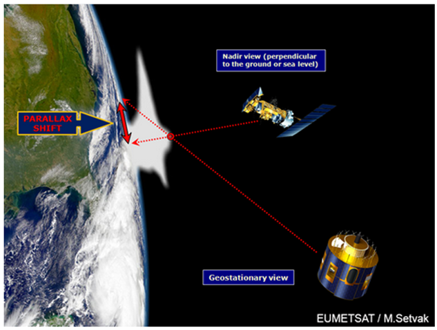
Figure 8: Illustration of parallax shift in satellite meteorology. 10
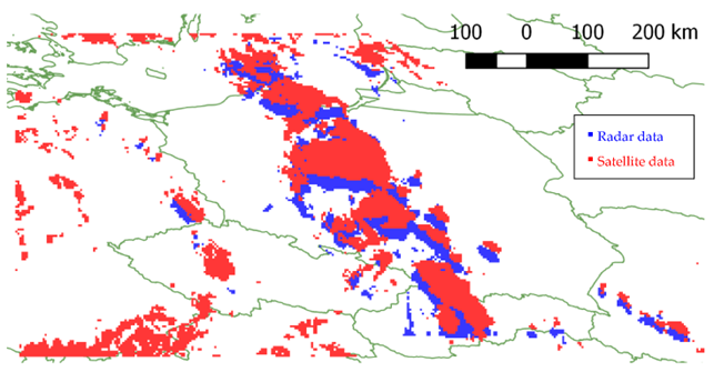
Figure 9: Illustration of parallax shift by comparing satellite and radar data. 3
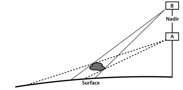
Figure 10: The viewing angle of the cloud from the LEO satellite (A) is greater than that of the GEO satellite (B). This leads to a larger displacement error for the cloud for the LEO satellite. 4
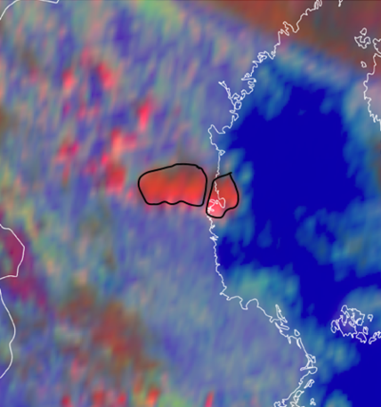
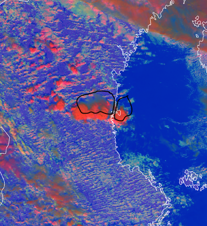
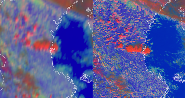
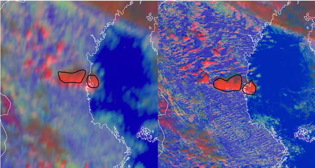
Figures 11, 12 and 13 illustrate the parallax shift phenomenon during the occurrence of a mesoscale convective system (MCS) in Finland in June 20215. Figures 11 and 12 compare the position of the cumulonimbus cloud as observed by a GEO satellite (SEVIRI, left image) and a LEO satellite (VIIRS, right image). The position of the cloud in the satellite images, taken approximately at the same time, varies due to its differing distance from the nadir. In the SEVIRI image, the position of the cumulonimbus cloud is shifted towards the northeast in comparison to the VIIRS image. Similarly, Figure 12 demonstrates a parallax shift of 45 km to the northeast.
Figure 13 compares the position of the cumulonimbus cloud as observed by two different LEO satellites (VIIRS and MODIS). This figure provides a further comparison of the position of the cumulonimbus clouds near the middle (red) and towards the edge (blue) of a polar satellite swath. With polar satellite imagery, the parallax effect becomes more pronounced towards the edges of imaging swaths. In addition, VIIRS exhibits a significantly reduced pixel growth rate from nadir to the end of the scan in comparison with the MODIS instrument.
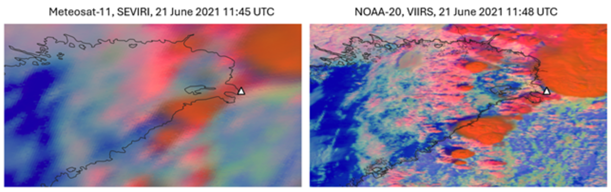
Figure 11: Day Microphysics RGB: 21 June 2021, around 11:45 UTC. Comparison between GEO (Meteosat-11, SEVIRI, left image) and LEO (NOAA-20, VIIRS, right image) satellite images. The city of Oulu is marked with a triangle.
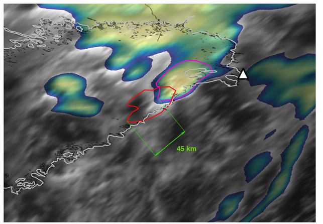
Figure 12: SEVIRI IR Sandwich product based on HRV channel: 21 June 2021, 10:00 UTC. The red contour shows the Cb cloud position in VIIRS (LEO satellite) and the magenta contour in SEVIRI (GEO satellite). The city of Oulu is marked with a triangle.
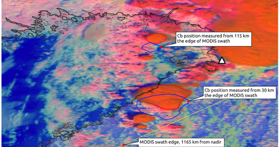
Figure 13: Day Microphysics RGB (NOAA-20, VIIRS): 21 June 2021, 11:48 UTC. Comparison of Cb clouds positions between the middle of a polar satellite swath (red lines) and the edge of a swath (blue lines). The city of Oulu is marked with a triangle.
The displacement due to parallax can also result in distortion of the shape of the original feature, whereby it is perceived to be larger or differently shaped than it actually is. Furthermore, the pixel size is relatively stretched in the scanning direction (Figure 14), which results in a feature appearing longer in the satellite image than it actually is in nature. As previously discussed, the satellite occasionally measures the sides of convective clouds rather than their tops at high latitudes, which can lead to inaccuracies in data interpretation. This is because the sides of clouds can present different characteristics from their tops, such as different temperatures.
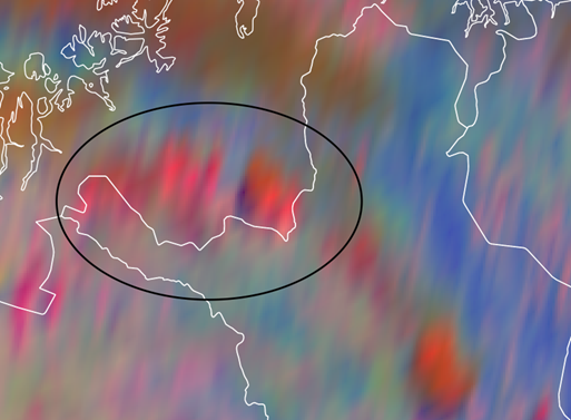
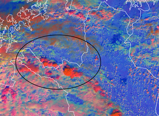
Figure 14: Day Microphysics RGB (SEVIRI and VIIRS): 29 June 2024, 09:45 UTC and 09:38 UTC
Exercise 2
Scenario
Consider a hypothetical work shift during the summer months, with the forecast indicating the possibility of convective showers in the central part of Sweden during the afternoon hours. Unfortunately, the radar is dysfunctional today, so for nowcasting the meteorologist has to rely on satellite imagery, SYNOP observations and NWP model data. The image below is a SEVIRI satellite image of a small convective cell.
Task:
1) Draw the border of the convective cell.
2) Do you recall the direction of the parallax, is it towards the south or towards the north?
Exercise 3
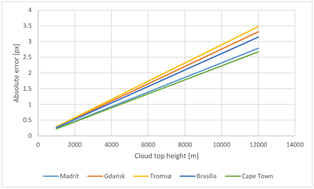
As we have discussed in this learning module, parallax shift is a problem in high-latitude regions. How can you explain the result shown in the figure below? Why is parallax shift larger in Brasília than in Cape Town, even though Brasília is closer to the equator?
Your answer:
Limb Cooling
Limb cooling occurs when the radiation travels through a longer path in the atmosphere at slanted viewing angles in comparison to the nadir path, resulting in increased absorption for a given wavelength. Absorption occurs especially by ozone and carbon dioxide, in so called absorption channels. In contrast, atmospheric window channels are regions in the electromagnetic spectrum where the Earth's atmosphere absorbs very little radiation, thereby allowing most of the radiation to pass through.
Because of limb cooling, the colors in RGBs change towards the edges of imaging areas. This color distortion can complicate the interpretation of satellite images: for example, in the Airmass RGB it can make it harder for a forecaster to locate jet streams or areas of cyclogenesis. In Figure 15, it can be seen that the color contrast between purple and red tones becomes weaker farther north. This is because at lower viewing angles there is more absorption at the wavelengths set to the red color beam than at less slanted viewing angles farther south.
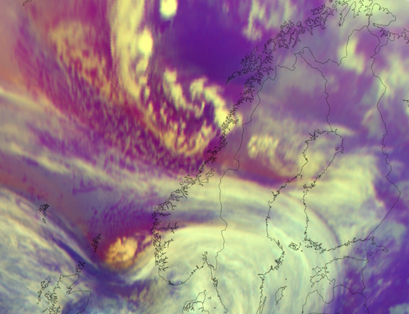
FIgure 15: SEVIRI Air Mass RGB: 04 April 2022, 07:15 UTC
If IR measurements farther away from the nadir are compared between window and absorption channels, a given cloud top or surface always appears colder in the absorption channels. This is most noticeable in the hues of water vapor RGB images and near the edges of full disk Airmass RGB images, as shown in Figures 16 and 17. It is also worth noting that limb cooling is not just a high-latitude problem: for example, it can be observed in the image in northwestern parts of Brazil. In water vapor imagery the edges of the disc appear drier than they really are due to low satellite viewing angles and therefore longer optical paths.
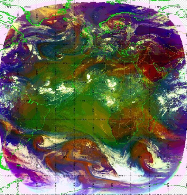
FIgure 16: SEVIRI Airmass RGB Full disc: 02 September 2024, 09:00 UTC
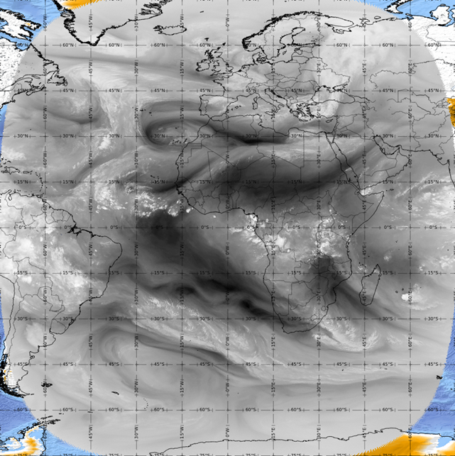
Figure 17: SEVIRI WV 6.2 microns Full Disc: 21 November 2024, 09:00 UTC
In the Airmass RGB the green beam is set to be the difference between the IR 9.7 and IR 10.8 channels (Figure 18). The slanted viewing angle at the edges of the full disk image reduces the radiation measured at 9.7 μm, while the window channel at 10.8 μm remains largely unaffected, and a larger (negative) brightness temperature difference results in a smaller green contribution. Limb cooling can also be seen in the edges of the imaging swath of a polar orbiting satellite in Figure 19 (here over western Russia for example), but for polar satellites the phenomenon is not as strong as for GEO satellites, because the distance to the edge of an image swath is smaller than the distance to the edges of an image disk.
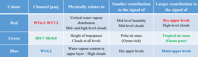
Figure 18: Air Mass RGB recipe for SEVIRI
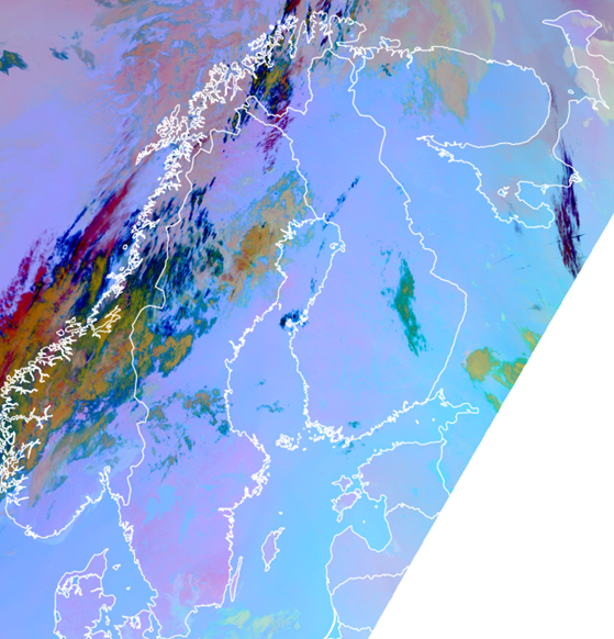
Figure 19: VIIRS Day Microphysics RGB: 26 June 2024, 02:24 UTC
Exercise 4
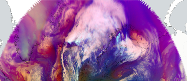
SEVIRI, Full Disc (cropped to high latitudes), 7 November 2024, 11:00 UTC
Why does the color in the Airmass RGB turn blue/purple at high latitudes at slanted satellite viewing angles?
Short wave visible channels
When using satellite products that contain short-wave visible channels, it can sometimes be easier to see certain phenomena or features better at high latitudes, due to the longer optical path. For example thin cirrus clouds, dust and smoke are more easily visible at high latitudes because the scattering from the aerosols within a thin layer of ice crystals or a sparse cloud of smoke or dust is stronger than for shorter optical paths.
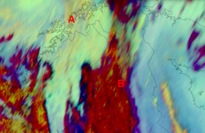
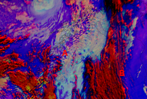
Figure 20 illustrates how thin cirrus clouds are better visible in GEO satellite images in comparison to polar satellite images. This is due to the light taking a longer path through the atmosphere containing such clouds to the GEO satellites. The difference can best be seen by comparing the images in the Day Microphysics RGB product between the SEVIRI and VIIRS instruments. In the SEVIRI image the cloud can be clearly seen over Swedish and Finnish Lapland (the northern parts of these countries) whereas from VIIRS the signal is very weak. In fact, in VIIRS it is possible to mistake the cloud signal for something else, such as terrain features.
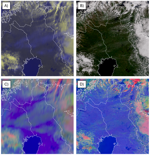
Figure 20: Comparison of cirrus clouds over Finnish Lapland, 27 June 2024 for different satellite products: A) SEVIRI HRV Clouds RGB, 10:15 UTC B) VIIRS True Color RGB, 10:16 UTC C) SEVIRI Day Microphysics RGB, 10:15 UTC and D) VIIRS Day Microphysics RGB, 10:16 UTC.
Resolution
A GEO satellite orbits at an altitude of approximately 36,000 km, allowing it to remain stationary over a specific longitude along the equator6. To ground observers, the satellite appears to be fixed in one position in the sky. The larger distance from the Earth's surface means that its sensors capture images with less detail. In addition to the increased distance, GEO satellites often observe objects on Earth at a slanted angle, resulting in further degradation of the resolution (Figure 3). Reduced resolution at high latitudes has many disadvantages: convection monitoring becomes more difficult, broken cloudiness is harder to observe during both daytime and nighttime and it can become impossible to discern some smaller scale features such as valley fog using, e.g., only geostationary data from the SEVIRI instrument. The newer FCI instrument on MTG (Meteosat Third Generation) has a higher resolution than that of SEVIRI and the difference between the old and new imagery is especially noticeable at high latitudes. The nominal spatial resolution of SEVIRI channels used in the Day Microphysics RGB is 3 km whereas with FCI it is 1 km.8 An example of this is presented in Figure 26, which depicts low-level clouds and fog over central Finland during the morning hours. The extent of the fog is more distinctly discernible in the FCI imagery. Furthermore, the movement of advection fog beneath overlying partial cloud layers may be traceable, providing potentially critical information for airport operations.
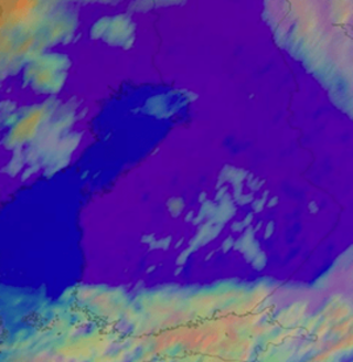
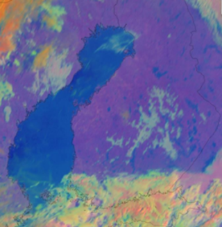
Figure 26: SEVIRI and FCI Day Microphysics RGB - 16 September 2024, 07:00 UTC
Polar satellites orbit at an altitude of approximately 800 km and are in constant motion relative to ground observers7. In polar satellite images, objects are closer to nadir than for GEO satellites, but the closer the objects are to the edge of an image swath, the poorer the resolution becomes. Polar satellites have higher spatial resolution, which is crucial for applications such as detailed environmental monitoring, land use mapping, and disaster management. In general, the choice between geostationary and polar satellites depends on the specific needs of the forecaster. GEO satellites are ideal for continuous, real-time monitoring of developing weather situations, despite their lower resolution.
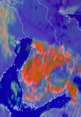
An illustrative example of resolution differences due to latitude can be seen below in Figures 27 and 28. In both cases convection is taking place, but only at lower latitudes it is possible to discern cloud top features using geostationary data from the SEVIRI instrument, which makes it harder for a forecaster to assess the severity of the developing weather situation. The approximate pixel sizes for the locations in this example are shown below in Figure 29.
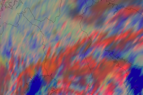
Figure 27: SEVIRI Day Microphysics RGB: 11 June 2024, (Northern Fennoscandia)
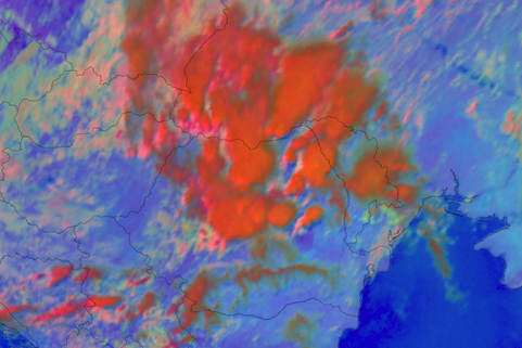
Figure 28: SEVIRI Day Microphysics RGB: 11 June 2024, 13:45 UTC (activity mainly over Romania and Ukraine)
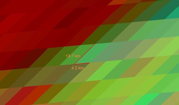
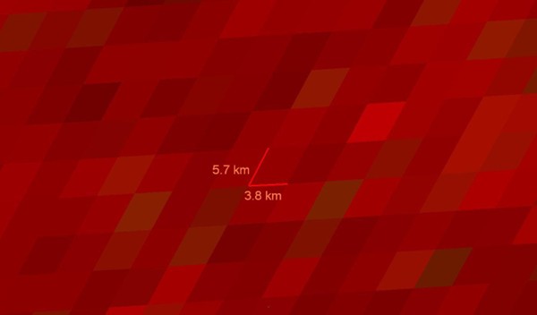
Figure 29: Comparison of SEVIRI pixel sizes (nominally 3x3km) in approximate locations of the convection in Figures 27 (Finland: 65.84N 24.13E) and 28 (Romania 46.10N 24.90E)
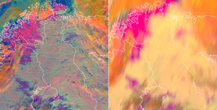
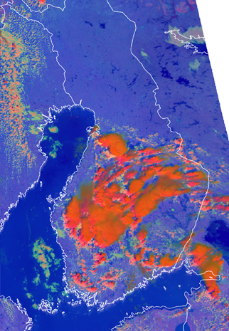
Figure 30: Day Microphysics RGB: 25 February 2024, VIIRS 11:38 UTC, SEVIRI 11:45 UTC (Northern Finland)
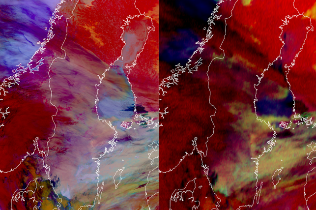
Figure 31: Night Microphysics RGB- 12, February 2024, VIIRS 01:42 UTC, SEVIRI 01:45 UTC (Central Sweden)
Another example illustrating resolution differences can be seen in Figure 30: looking at the clouds in the northeastern parts of Sweden, it is obvious that in this case it is difficult to tell where broken cloudiness is situated using only SEVIRI data, whereas in VIIRS data more exact locations can be observed. Observing broken cloudiness is especially important in winter when the road surface is at risk of freezing, because broken clouds lead to faster radiative cooling of a surface compared to overcast conditions. An example of this can be seen in Figure 31, where the lower cloud cover breaks in central parts of Sweden, but it is quite difficult to observe from SEVIRI data because the clear areas are quite small and there is also some higher cloud over the lower cloudiness.
Exercise 5
VIIRS has better spatial resolution than SEVIRI. Which cloud top features can be more easily distinguished using VIIRS imagery?
Use the slider.
|
|
Exercise 6
Scenario:
Imagine you receive a phone call in mid-September from a customer asking whether it is safe to drive from Destination A to Destination B the following night using summer tires.
Background:
Yesterday evening, a precipitation area passed over northern Sweden, causing widespread wet road surfaces. The NWP models are predicting minimum temperatures down to +2 degrees Celsius over higher terrain, together with light winds from the north. Accurate forecasting of cloud cover is crucial in this situation.
Task:
Using only SEVIRI satellite imagery, how would you assess the likelihood of:
- Broken cloud cover and freezing road surfaces during the night within the marked area?
Please explain your reasoning based on the satellite data available.
SEVIRI Night Microphysics RGB - 11th September 2024
Your answer:
How about now?
FCI Night Microphysics RGB - 11th September 2024
Your answer: