Physical background
In this chapter the physical characteristics of the Cloud Phase RGB channels are discussed. Table 2.1 shows which channels are used in the Cloud Phase RGB. Both NIR2.25 and NIR1.6 are microphysical channels, which provide information on cloud top phase and effective particle size in different ways. Using them together enables a reliable separation between thick ice and water clouds (explanation below). Effective particle size is a special kind of weighted mean of the particle sizes.
Note that for the red and blue colour beams the same channels as in the Natural Colour RGB are used. While the Natural Colour RGB focuses on vegetation, the Cloud Phase RGB focuses mostly on cloud top microphysics.
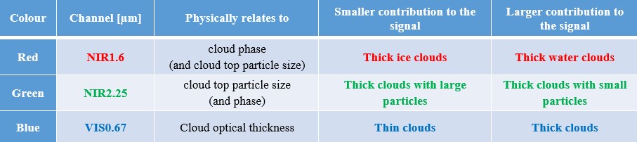
Table 2.1: Channels used in the Cloud Phase RGB
Fig. 2.1 shows the imaginary part of refractive index of water and ice as a function of wavelength on a logarithmic scale. This is the parameter that primarily defines the absorption: it can be seen that absorption is much weaker for wavelengths less than 1 µm, and that ice and water particles absorb differently.
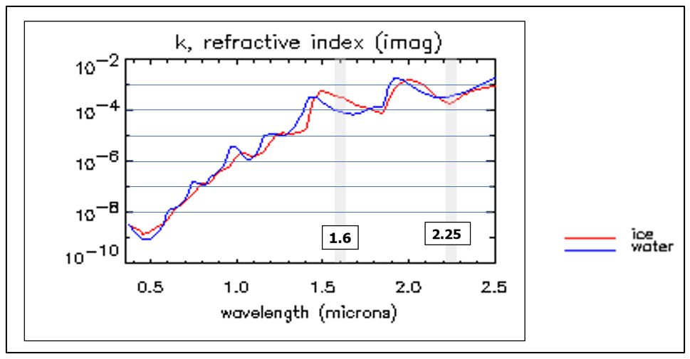
Fig. 2.1: Absorption of ice and water.
From Fig. 2.1 one can see that:
- The difference between ice and water absorption is less at NIR2.25 than at NIR1.6.
- The absorption of water is stronger at NIR2.25 than at NIR1.6.
- The absorption of ice is weaker at NIR2.25 than at NIR1.6.
- Absorption at VIS0.67 is negligible both for ice and water.
Cloud characteristics
When the wavelength is longer than about 1 µm, the reflectance of a thick cloud depends mainly on the cloud top microphysics (phase and effective particle size). When the wavelength is shorter than about 1 µm, the reflectance of thick clouds depends mainly on the optical depth, varying only slightly with changes in cloud top phase and effective particle size. This behaviour is shown in Fig. 2.2, presenting simulated reflectance of water clouds as a function of optical depth for several wavelengths and cloud top effective radius values.
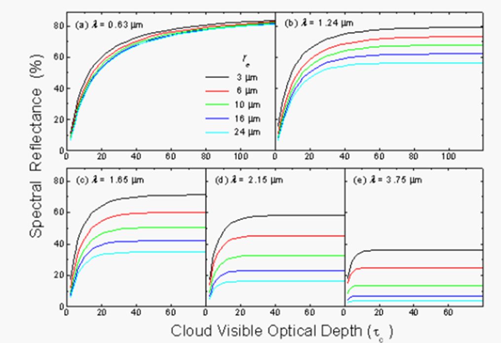
Fig. 2.2: Simulated reflectance of water clouds as a function of optical depth for several wavelengths and cloud top effective radius values. (Source: SlidePlayer)
Fig. 2.3 shows simulated albedo of opaque water and ice clouds for 1.6 µm (top) and 2.25 µm (bottom) as a function of radius (effective radius for water clouds and radius derived from averaged geometrical cross-section for ice clouds).
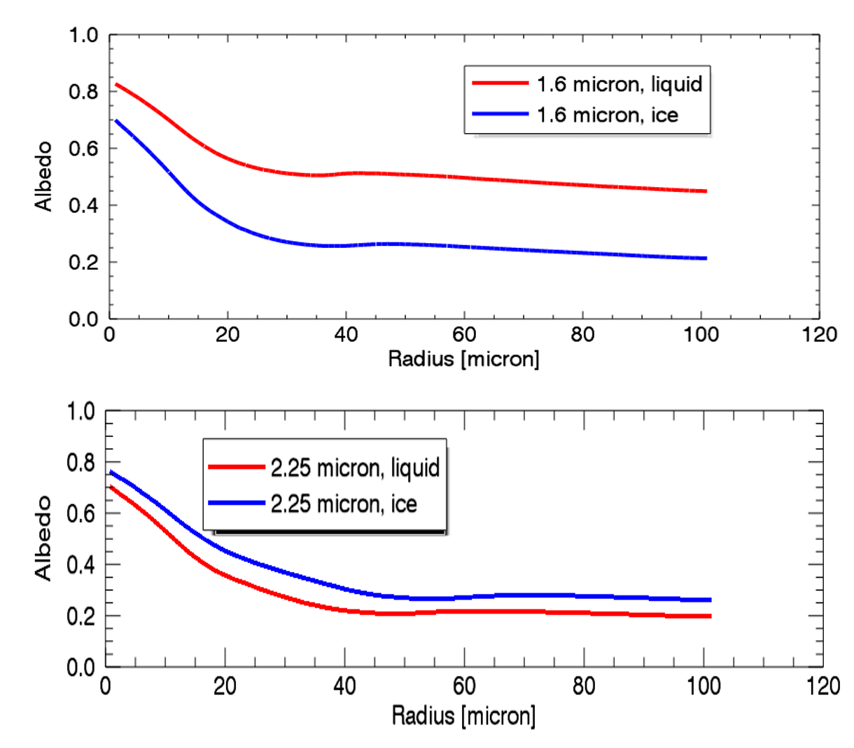
Fig. 2.3: Simulated albedo of opaque water and ice clouds for 1.6 µm (top) and 2.25 µm (bottom). (Source: Ralf Bennartz, University of Wisconsin-Madison)
From Fig. 2.3 one can see that:
- NIR1.6 data is usually good for separating opaque ice and water clouds, due to the large difference between the water and ice cloud albedo curves and the fact that the ice crystals on the ice cloud tops are typically much larger than the droplets on the water cloud tops. However, there are exceptions: ice clouds covered by small ice crystals and water clouds covered by large droplets can have similar albedo values.
- NIR2.25 alone is NOT good for separating phase, as the two curves are close to each other. However, it is good for separating opaque clouds with small and large particles. The NIR2.25 albedo changes over a broader interval of cloud top particle sizes than the NIR1.6 albedo.
To illustrate the above statements, we show an example over New Zealand (Fig. 2.4). In the VIS0.5 channel all opaque clouds are bright. In the NIR1.6 image there are bright and medium grey clouds with rather good contrast between them. Ice clouds are darker than water clouds. However, the encircled clouds are ice clouds, despite being rather bright. These are high-level lee clouds (cirrus clouds), which typically consist of very small ice crystals. In the NIR2.25 image there is less brightness contrast within the cloudy area. The high-level lee clouds are bright.
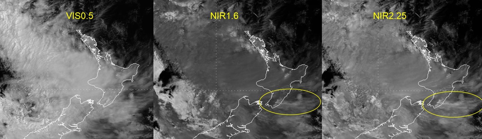
Fig. 2.4: Himawari/AHI VIS0.5, NIR1.6 and NIR2.25 images over New Zealand. The encircled clouds are high-level lee clouds.
The statement that NIR1.6 is usually good for separating opaque ice and water clouds (with some exceptions) is also confirmed by Fig 2.5. The left panel shows simulated VIIRS reflectance pairs (NIR1.6 and VIS0.64) for water and ice clouds over ocean. The blue curves correspond to ice clouds and the orange curves to water clouds. The simulated reflectance values depend on the optical depth (constant along the dashed lines), effective particle size (constant along the solid lines) and angles, as well as on the characteristics of the background (in the case of thin clouds). Such simulated values are used in optical depth and particle size retrieval with SEVIRI data. As there is some overlap between the orange and blue curves one cannot always unequivocally retrieve cloud top phase (and hence particle size) using this channel pair. This is also confirmed by measurements (see the right panel).
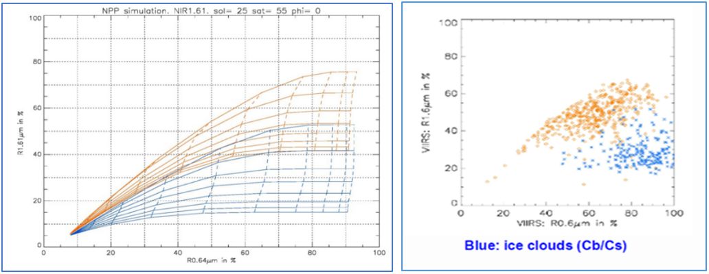
Fig. 2.5: Simulated (left) and measured (right) VIIRS NIR1.6 and VIS0.64 reflectance pairs for water and ice clouds over sea. Curves and symbols referring to water and ice clouds are orange and blue, respectively. Effective radius varies between 3 and 24 µm for water and 5 and 40 µm for ice clouds. Optical depth varies between 0 and 256. (Source: G.Kerdraon et al., Meteo-France, NWCSAF)
Fig. 2.5 confirms that combining NIR1.6 with VIS0.6 does not provide perfect separation between ice and water clouds. However, if we use the two microphysical channels (NIR1.6 and NIR2.25) together then we will have a more reliable, more perfect separation, see Fig. 2.6. That is why both microphysics channels are used in the Cloud Phase RGB.
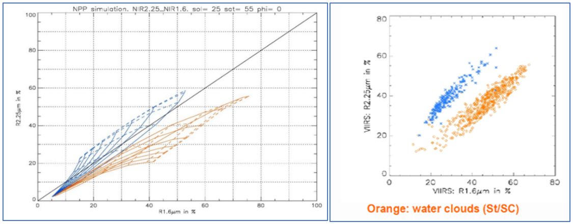
Fig. 2.6: Simulated (left) and measured (right) VIIRS NIR1.6 and NIR2.25 reflectance pairs for water and ice clouds over ocean. Curves and symbols referring to water and ice clouds are orange and blue, respectively. (Source: G.Kerdraon et al., Meteo-France, NWCSAF)
In the case of (very) thin clouds, the water and ice curves are close to each other (see the encircled area in Fig. 2.7.) In this region the cloud phase retrieval may be uncertain.
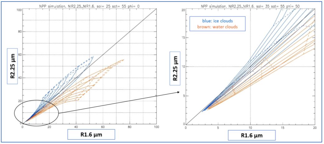
Fig. 2.7: Simulated VIIRS NIR1.6 and NIR2.25 reflectance pairs for water and ice cloud over ocean (left). A closer look at the encircled area (right) shows the thin clouds. Curves referring to water and ice clouds are orange and blue, respectively. (Source: G. Kerdraon et al., Meteo-France, NWCSAF)
Snow characteristics
The left panel of Fig. 2.8 shows snow reflectance spectra. The reflectance is high in the visible region and much lower at wavelengths above 1.4 µm. Snow is bright at 0.6 µm and rather dark at both 1.6 and 2.25 µm. (Snow detection is based on this behaviour.)
The snow reflectance also depends on the snow grain size: finer snow reflects more strongly. From the left panel of Fig. 2.8 one can see that the NIR2.25 channel is more sensitive to the snow grain size than the other two channels used in the Cloud Phase RGB. As a consequence, the Cloud Phase RGB will be more sensitive to the snow grain size than other RGBs using only the NIR1.6 channel.
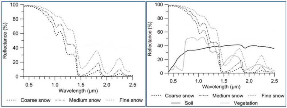
Fig. 2.8: Typical reflectance spectra of snow (left) and snow, soil and vegetation (right)
If the area is covered by thick clouds, we have no information about whether the surface is covered by snow. If the area is covered by thin clouds, then snow might be identified if the cloud is sufficiently thin (transparent). Animation may help in such cases.
Note that appearance of snow on satellite imagery depends not only on the snow characteristics (e.g., fresh/old, grain size, melting, pollution), but also on whether the pixel is totally covered by snow (snow patches, partly cleared snow, un/frozen patches of lakes and rivers, dark tree branches over the snow, shadows, etc.).
Sea and land characteristics
Fig. 2.9 shows the typical reflectance spectra of soil, green vegetation and water. The reflectance of deep water is negligible at 1.6 and 2.25 µm and not negligible but rather low at 0.6 µm. The typical soil reflectances at 1.6 and 2.25 µm are about the same, but are much weaker at 0.6 µm. The actual values depend on the soil type. The typical reflectance of green vegetation is strongest at 1.6 µm, weaker at 2.25 µm and weakest at 0.6 µm. The actual values depend on the vegetation type. The land pixels are often a mixture of soil and vegetation.

Fig. 2.9: Typical reflectance spectra of soil, green vegetation and water