Typical Appearance In Vertical Cross Sections
Here are some relevant NWP parameters that describe the vertical structure of Australian shallow cold fronts.
- Potential temperature contours give a good indication of the formation and strengthening of the front, as well as its depth thus verifying it as a shallow cold front. Wave features in the isentropes can reveal solitary waves travelling with or ahead of the front. In the case of Central Australian fronts the Potential Temperature can distinguish between a well mixed daytime boundary layer, the nocturnal regeneration of the Central Australian front as well as formation of the nocturnal inversion ahead of this.
- Equivalent potential temperature contours can distinguish between airmasses, permit the monitoring of airmasses that are being modified. Also permits analysis of atmospheric stability.
- Horizontal windspeed normal to the cross section. This reveals wind changes associated with the front, defining the front better. It also shows the development of the nocturnal jet in the case of the Central Australian front.
- Vertical velocity. Important in defining the location of the front, also the strength of the frontal updraft.
- Vorticity shows subtle features associated with the shallow cold fronts including pre-frontal solitons etc. Anticyclonic vorticity is important in defining the building of the ridge of high pressure accompanying the development of the Southerly Buster
- The Frontogenesis function, the Eddy exchange coefficient of momentum and convergence / deformation have also been used (not described here)
Note that station or model soundings are also very useful in identifying shallow cold fronts.
Equivalent Potential Temperature, Omega, Relative Humidity, Wind
|
|
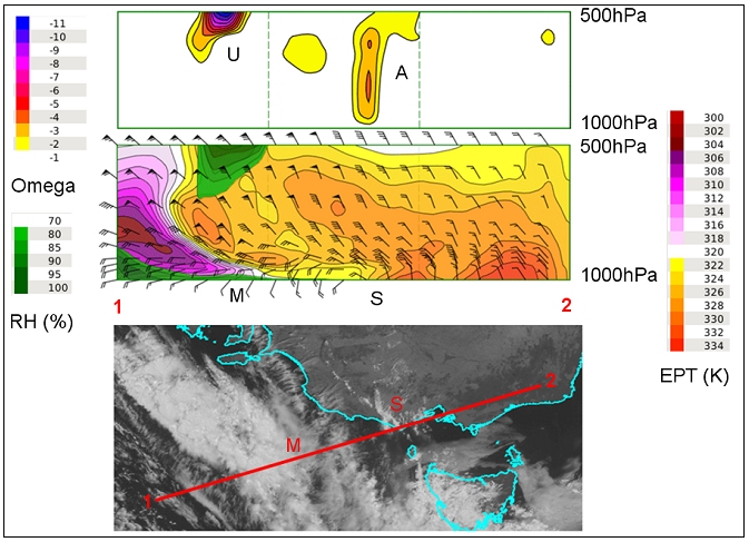
Figure 25: Parameters: Equivalent Potential Temperature, Omega, Relative Humidity, Wind. Images courtesy JMA and BOM
|
Cross-section across the shallow cold front of 17th January 2014 along the axis 1-2 showing variations in vertical motion (omega) in the top diagram, equivalent potential temperature, relative humidity and wind direction and strength in the middle diagram and the corresponding visible satellite image. S shows the nose of the shallow cold front, M is the head of the Southern Ocean front. A is the vertical motion associated with the shallow cold front and U with the Southern Ocean front.
Potential Temperature, Vertical Motion
|
|
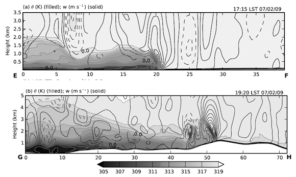
Figure 26: Parameters: Potential Temperature, Vertical Motion Images from Engel et al. 2012
|
Cross section of potential temperature (shaded) and vertical motion of the Black Saturday (Type 2) shallow cold front as it makes landfall at Melbourne and as it interacts with the topography of the Great Dividing Range.
Potential Temperature, Vertical Wind Speeds
|
|
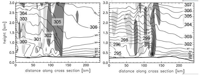
Figure 27: Potential Temperature, Vertical Wind Speeds Images from Thomsen et al. 2009
|
Central Australian Fronts. (LHS) 06EST on 10 September 1991 (RHS) 06EST on 17 September 1991. Potential temperature (K) and vertical wind speeds greater than 10cm/s (dark), and less than -10cm/s (light). The fronts are moving from left to right with the strongest upward motion at the head of the front. Note that the Central Australian Front of the 10 September 1991 (LHS) has amplitude ordered solitary waves travelling with the front.