Table of Contents
Cloud Structure In Satellite Images
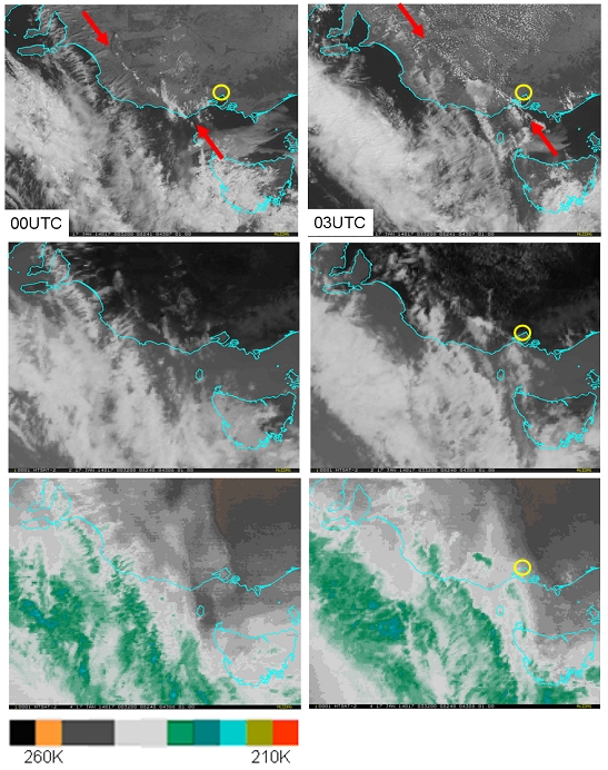
The shallow cold fronts propagate within environments that generally have very limited amounts of atmospheric moisture. Type 2 fronts and Southerly Busters are best observed in the visible images due to shallow nature of front and the associated low-level cloud. The Central Australian Front is commonly tracked at night using enhanced infrared imagery. Progression of the fronts over the maritime regions may be monitored using satellite microwave scatterometer data.
The Type 2 shallow cold front which crossed western parts of Victoria, Australia on the 17 January 2014 at times 00UTC and 03UTC is annotated by red arrows and shown in the visible (top), infrared (middle) and enhanced water vapour imagery (bottom). Clearly the visible image is the best for viewing this feature, though the infrared image may be useful at night. The location of the city of Melbourne is shown as a yellow circle.
Schematic diagrams of cloud signatures of three EXCY episodes are shown below.
|
|
|
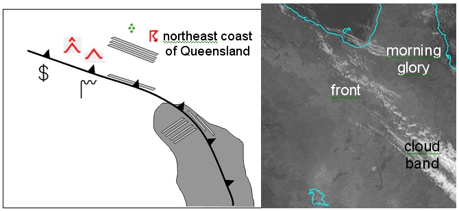
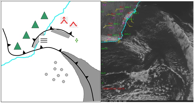
Figure 2 & 3: Schematic and satellite image of the cloud signatures and other features of a Type 2 front. Courtesy of Japan Meteorological Agency (JMA) and Australian Bureau of Meteorology (BOM)
|
|
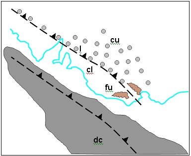
Schematic of the cloud signatures and other features of a Type 2 front that can be detected in satellite imagery.
| Dc | deep cloud associated with the weakening Southern Ocean front (visible, infrared, water vapour) |
| Fu | smoke plumes from bushfires that change direction as the Type 2 front crosses the location (visible, sometimes infrared). |
| Cu | cumulus cloud can sometimes be seen upstream of this front (visible, infrared) |
| L | a line of cumulus cloud can sometimes be seen associated with this front (visible, infrared) |
| Cl | mostly clear of cloud on land behind the front |
|
|
|
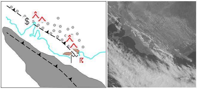
Figure 4: Schematic of the cloud signatures of a Southerly Buster.
|
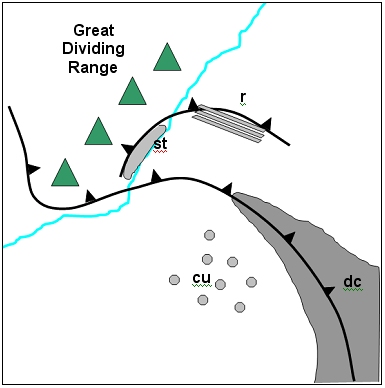
Schematic of the cloud signatures of a Southerly Buster that can be detected in satellite imagery.
| Dc | deeper cloud associated with the cold front (visible, infrared, water vapour) |
| St | low cloud banking up against the escarpment of the range behind the Buster (visible, sometimes infrared). |
| r | roll clouds may be associated with the buster. (visible, sometimes infrared) |
| Cu | speckled cumulus cloud behind the cold front (visible, infrared) |
|
|
|
Figure 5: Schematic of the cloud signatures and other features of a Central Australian Front that can be detected in satellite data.
|
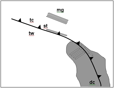
Schematic of the cloud signatures and other features of a Central Australian Front that can be detected in satellite data.
| Tc | cooler temperatures at night ahead of the front (infrared) |
| Tw | warmer temperatures at night behind the front (infrared) |
| Mg | morning glory cloudlines ahead of the front and near the Gulf of Carpentaria (visible) |
| St | low cloud associated with the front during the day (visible) |
| Dc | deeper cloud associated with the original Southern Ocean Cold Front over eastern Australia (visible, infrared, water vapour) |
Type 2 front in various satellite channels/products
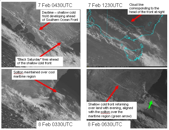
The evolution of the Type 2 front corresponding to the “Black Saturday Bushfire” event is shown in visible and infrared imagery below. A line of cumulus marks the region of surface convergence and frontogenesis. The broad cloudband corresponding to the Southern Ocean front is seen to the southwest. The eastward progression of the shallow front can thus be monitored using visible imagery during the day and infrared imagery during the night, provided there is sufficient low level moisture available to maintain the cloud line along the nose of the front. In the 0430 UTC image shallow cumulus cloud streets may be observed to develop in the warm northwesterly airstream ahead of the front. Note that the front cannot be detected over land at 0330UTC on the 8th February presumably due to the mixing of dry air through the deep daytime continental boundary layer. However, its progress may be followed over the adjacent maritime region as low level stratiform cloud associated with the passage of a solitary wavetrain.
Note that there is an absence of cloud in the cool and stable post-frontal region.
|
|
|
Figure 6: Evolution of a Type 2 shallow cold front, Black Saturday fire event, 7-8 February 2009 in visible and infrared (1230UTC) MTSAT-1R imagery. Images courtesy JMA and BOM
|
Southerly Buster
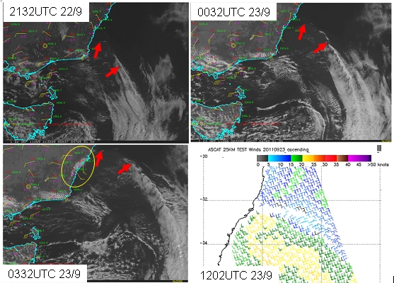
As shown in the figure below, the location of the parent cold front to the Southerly Buster can be clearly seen in satellite imagery as a sharply defined cloud line embedded within the frontal band and located in the Tasman Sea to the east. Closer to the east coast of Australia the dry continental westerly offshore flow is suppressing cloud formation. However, a wave train of solitary waves or a single roll cloud may sometimes be seen at the head of the Buster in the visible image though this is not so clear in the corresponding infrared image.
In the 0332UTC image the passage of the Buster can also be detected by the stratus cloud banking up against the ranges in the cold air behind the change as shown within the yellow circle. Microwave scatterometer data such as ASCAT and WindSAT is also useful in monitoring the progress of the Buster, however this polar orbiting satellite data has limited temporal frequency.
|
|
|
Figure 7: Cloud features associated with the Southerly Buster of 23 September 2011, MTSAT-1R visible imagery and ASCAT scatterometer winds. Red arrows indicate the leading edge of the Buster. The low cloud banking up against the escarpment behind the passage of the Buster is located within the yellow ellipse. Images courtesy JMA and BOM, bottom right image courtesy NOAA/STAR
|
Central Australian fronts
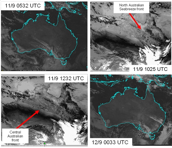
Central Australian fronts are best detected during the night when the fronts have the strongest intensity and the most pronounced signal in the infared channel. Inspection of an animated loop of this imagery defines the front as dividing the cooler nocturnal inversion ahead from the warmer turbulent boundary layer behind the front. “Southern Morning Glories” travelling ahead of the front may be detected using the visible channel during the daytime.
|
|
|
Figure 8: Cloud features associated with the Southerly Buster of 23 September 2011, MTSAT-1R visible imagery and ASCAT scatterometer winds. Red arrows indicate the leading edge of the Buster. The low cloud banking up against the escarpment behind the passage of the Buster is located within the yellow ellipse. Images courtesy JMA and BOM, bottom right image courtesy NOAA/STAR
|
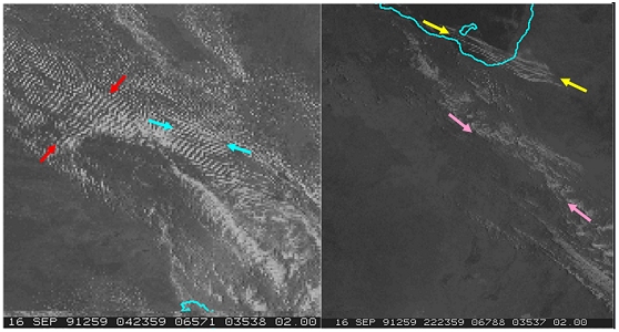
In the visible daytime images shown above it can be seen that the band of cloud associated with the higher latitude front may persist over southern and eastern parts of the continent as the Central Australian front moves northwards. The progression of this can be followed in the visible and infrared images. Cloud streets oriented parallel to the direction of boundary layer wind shear can be seen in the visible images shown below.
|
|
|
Figure 9: Cloud features associated with Central Australian front event of the 16th September 1991. Images courtesy JMA and BOM
|
Left-hand side: pre and post frontal cloud streets, blue arrows show pre-frontal cloud streets oriented in a northwesterly direction, red arrows indicate post frontal cloud streets oriented in a southwesterly direction. Right-hand side: the cloud features on the following morning. Yellow arrows annotate the solitons (Morning Glory), pink arrows indicate the approximate position of the surface front. GMS-5 visible imagery.
|
|
|
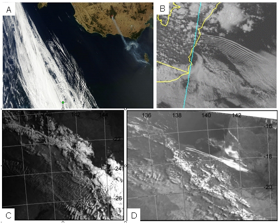
Figure 10: Solitary waves and wave-trains associated with different cold fronts. Top left image courtesy NASA/GSFC Rapid Response, top right image courtesy JMA and BOM, bottom images from Thomsen et al. 2009
|
Solitary waves and wave-trains associated with different cold fronts:
A: ahead of a Southern Ocean front, 18 February 2013 0030UTC Terra MODIS image.
B: associated with a Southerly Buster, 7 January 2009 MTSAT-1R visible image.
C: associated with a Central Australian front, propagating with the front 10 September 1991 0818EST NOAA-12 AVHRR image.
D: associated with a Central Australian front, propagating ahead of the front as a 'Morning Glory' 17 September 1991 0730EST NOAA-12 AVHRR image.
Meteorological Physical Background
The interaction of a Southern Ocean cold front or oceanic trough or coastal low with the Australian continent is the important process for the generation and maintenance of Australian shallow cold fronts. The enhancement of strong temperature contrasts between land and ocean during summer generates Type 2 fronts, the interaction of the cold front with the Great Dividing Range generates the Southerly Buster. Nocturnal boundary layer processes over the arid Australian interior maintain the Central Australian front.
|
|
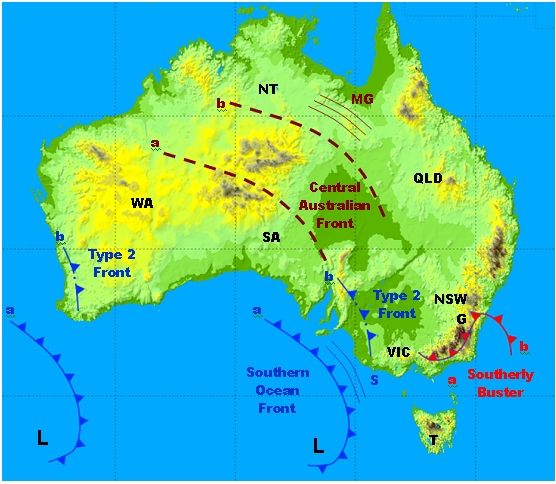
Figure 11: Summary of the Type 2 front, the Southerly Buster and the Central Australian front.
|
Summary of the Type 2 front, the Southerly Buster and the Central Australian front. Progression of the fronts is annotated as a-b. Also shown are Southern Ocean low pressure centres (L), solitary wave trains that propagate ahead of a Southern Ocean front (S) and Southern Morning Glories travelling ahead of a Central Australian front (MG). Australian states are Victoria (VIC), New South Wales (NSW), Queensland (QLD), South Australia (SA), Western Australia (WA), Northern Territory (NT) and Tasmania (T). The Great Dividing Range (G) is also shown.
Broad Overview
Type 2 summer cold front
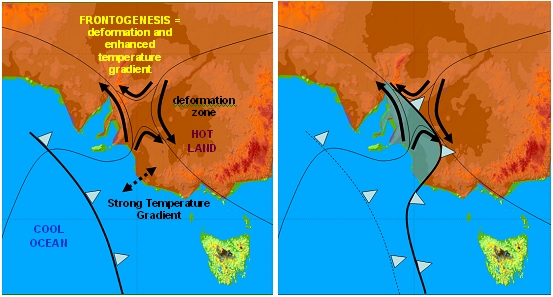
A schematic showing the mechanism of genesis of Type 2 fronts ahead of an approaching Southern Ocean front is shown below. This may involve an interaction between the front and the summertime heat trough located over continental Australia. The temperature contrasts between the cool ocean and the hot continent is enhanced by the low level wind field within the deformation zone of the heat trough. This mesoscale frontogenesis is particularly pronounced along and inland of the east coast of South Australia and Victoria where the coastline is near parallel to the approaching front. It has also been observed inland of southwestern parts of the continent (Western Australia).
This frontogenesis generates the Type 2 front with a weakening of the Southern Ocean front upstream. This can result in an apparent "jump" in the progression of the change, with the front typically traversing coastal regions between late morning and early evening.
|
|
Figure 12: Development of the Type 2 fronts. LHS during the day, RHS front replacement during the evening.
|
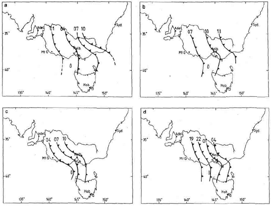
The lifecycle of four Type 2 cold fronts are shown below. In all cases genesis occurs inland from the east coast of South Australia and Victoria. Eastward propagation is more rapid over the maritime region so the front deforms in shape. The fronts shown here dissipated over inland Victoria / southern New South Wales, though on occasions this system may interact with the mountains of the Great Dividing Range and evolve into a Southerly Buster.
|
|
Figure 13: Isochrones of four 'Type 2' cold fronts crossing southern Victoria and Bass Strait. (a) 8 February 1983, (b) 16 February 1983, (c) 14 January 1985, (d) March 1986. Images from Garratt 1988
|
As these fronts typically occur during the latter part of summer there is generally little atmospheric moisture available so only shallow cloud may define the front. The fronts have similarities to an unsteady shallow gravity current. A very strong cold front with the structure of a gravity current is shown below. Note the relative flow of cold air towards the leading edge and strong ascent at the head of the front.
|
|
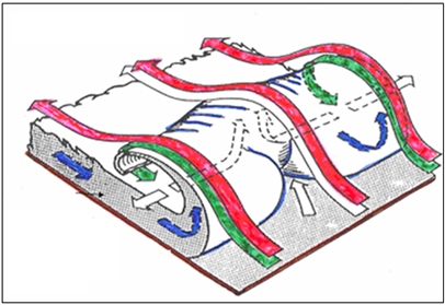
Figure 14: Schematic of a Type 2 summertime front. Very shallow surface cold air flows towards the leading edge (blue arrows). Circulation at the head of the current is shown with entrainment of pre-frontal air (green arrows). Image from Tepper 1950
|
"Southerly Buster"
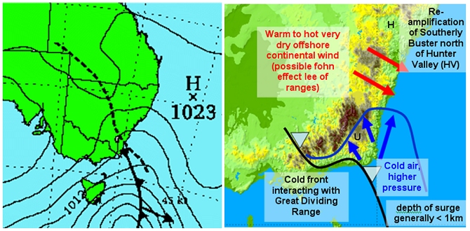
A Southerly Buster is the result of a cold front which interacts with topography, specifically the Great Dividing Range of southeastern Australia. This results in the channelling of the cool maritime air around the southeastern part of the mountain ranges and the blocking of the flow on the western side of the mountains. The upslope flow on the southern and eastern flank of the ranges induces anticyclonic turning of the winds resulting in a ridge of high pressure behind the cold front. A schematic of a Southerly Buster on the synoptic and mesoscale is shown below.
|
|
Figure 15: Schematic of the Southerly Buster on the synoptic and mesoscale. Upslope flow resulting in anticyclonicity and strengthening of the ridge of high pressure (U).
|
Many of the fronts classified as "Southerly Busters" are not southern ocean fronts but had formed on the pre-frontal trough south of the continent or appeared to originate on the southern NSW coast in association with shallow mesoscale low development. The lifespan of the Buster is generally less than 24 hours from the time the cold front reaches the Great Dividing Range in southern NSW to its dissipation on the north coast or southern coast of Queensland.
As the Southerly Buster progresses northwards the strength and depth of the surge decreases, however in some cases the Buster strengthens north of the Hunter valley. This is due to upslope flow north of the valley permitting the flow to acquire anticyclonic vorticity in a manner similar to the original blocking and formation of the Southerly Buster in Victoria.
|
|
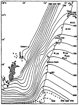
Figure 16: Isochrones showing the progression of the Southerly Buster from 06EDST 25 November 1982 to 01 EDST 26 November 1982.Image from Colquhoun et al. 1985
|
The Buster advances into a strongly stable boundary layer with warm summertime prefrontal continental air advecting over a cooler sea. This may results in a roll vortex which extends ahead of the cold front in about half of the observed Busters. The gravity current head breaks away from the feeder flow supplying it with cold air as shown in the diagram below. In this way the Buster does not behave like a gravity current. The pre-frontal boundary layer is between 100 and 200 metres deep and if the pre-frontal stable layer is deep and strong, the roll vortex will evolve as a solitary wave type disturbance or as a bore wave that propagates on the stable layer.
|
|
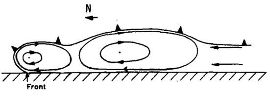
Figure 17: The Southerly Buster frontal structure in cross section
|
The Southerly Buster frontal structure in cross section parallel to the coast for the event of the 11th December 1972. Streamlines represent airflow relative to the circulation centres of the roll vortices and straight arrows indicate wind direction. The first circulation cell corresponds with the 28 minute period following the first wind change and the second cell with the subsequent two hour period.
Central Australian Fronts
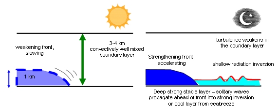
During the colder months cold fronts often penetrate across the Australian continent, sometimes reaching the northern shores of the continent at the Gulf of Carpentaria. These fronts are generally no deeper than about 1km and they advance into a convectively well mixed boundary layer, typically 3-4 km deep that overlies a strong shallow radiation inversion during the night.
Central Australian fronts are strongly modulated by the diurnal cycle with frontogenesis confined to the boundary layer, indeed. In particular the fronts weaken and decelerate after sunrise and strengthen and accelerate in the evening.
During the day two processes result in frontolysis. Firstly, radiative heating and associated turbulent mixing act to decelerate the low level winds which results in a reduction in the deformation and convergence. Secondly the air in contact with the heated surface is rapidly mixed through the boundary layer which is inversely proportional to the depth of the layer. Hence the shallow cold side of the front warms faster than the deep and well mixed boundary layer on the warm side of the front resulting in a decrease in the temperature contrast across the front.
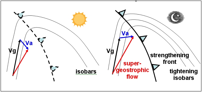
After sunset the front redevelops rapidly and accelerates once the boundary layer turbulence moderates. Decoupling between the atmosphere and the surface occurs with the reduced low level friction. This causes the ageostrophic wind vector to rotate anticlockwise (in the Southern Hemisphere) due to the removal of friction and the resultant unbalanced Coriolis force. This inertial oscillation results in supergeostrophic winds and as these low level winds strengthen so do the contributions made to frontogenesis by deformation and convergence, as shown in the figure below.
|
|
Figure 17: Schematic showing the diurnal modulation.
|
Schematic showing the diurnal modulation in the strength of the Central Australian front. The geostrophic wind vector (Vg) is shown as well as the development of supergeostrophic cross-isobar flow due to the anticlockwise rotation of the ageostrophic wind vector (Va).
In the early stages, whilst the front is over South Australia, there is normally an inland heat trough over northeastern Queensland. As the front progresses eastwards the frontal trough and heat trough merge.
As the front strengthens and encounters the developing radiation inversion and cool air advected inland by the sea breeze from the Gulf of Carpentaria to the north, "Southern Morning Glories" are observed to develop during the early hours of morning. These propagates upon the radiation and/or sea-breeze inversion ahead of the air-mass change and develop a series of large-amplitude waves at the leading edge as shown in the right hand panel in the diagram below.
|
|
Figure 18: Central Australian front during day (left) and during night (right). Also showing the development of a "Southern Morning Glory" on pre-frontal inversion.
|
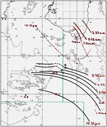
Of the 15 fronts observed during the field experiments starting in 1988 and extending over 10 years, 13 crossed central Australia during the evening or early hours of the morning. These fronts normally cross the continent from south to north within a day or two
|
|
Figure 19: Isochrones showing the progression of the Central Australian front of 11 September 1996. Image from Deslandes 2002
|
Geographical Location
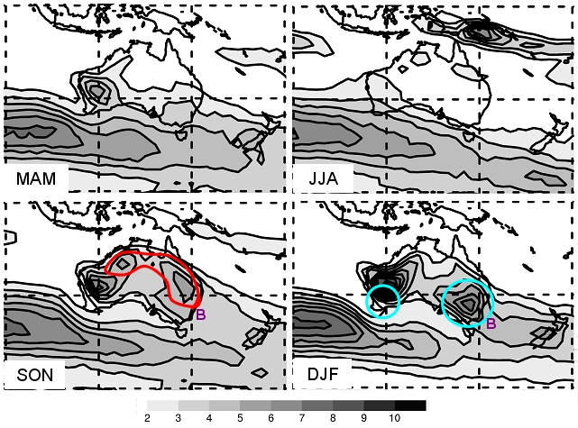
The figure below the climatology of cold fronts divided into three-monthly subsets. The frequency of cold fronts in the region is largest in summer with pronounced local maxima over southwestern and southeastern Australia. These maxima are distinct from the maxima to the south of the continent over the Southern Ocean. This indicates frontolysis of Southern Ocean fronts as these approach the Australian continent, with regeneration over the continent as predominantly Type 2 summertime shallow cold fronts. The distribution of central Australian fronts can be seen in the climatology for the spring months of September, October and November. Southerly Busters occur predominantly along the southeast coasts of the continent, specifically the east coasts of Victoria and New South Wales. It is possible that these Busters also affect the east coast of the island of Tasmania to the south of the Australian continent, as the orientation of the coast and the topography has similarities to the aforementioned coastline.
|
|
Figure 20: Mean seasonal evolution of cold front frequency for March to May (MAM), June to August (JJA), September to November (SON) and December to February (DJF). Units are percentage of time at which an objectively identified front was located within each 2.5 degree grid box during these months
|
Red outline shows frontal features over central and northern Australia, blue outline shows Australian summertime cold fronts, which tend to be predominantly Type 2 during the months December to February. The location of Busters is indicated as "B".
Key Parameters
Examination of published literature indicates that the following NWP parameters are important in detecting and nowcasting Australian shallow cold fronts.
- Surface pressure. Surface pressure minima define the location of the continental pre-frontal trough. The diurnal variations in the Central Australian front and its interaction with the Queensland heat trough can be monitored. The strong pressure gradient at the head of the Southerly Buster can be monitored.
- Surface and low level wind speed and direction. Changes in wind direction define the nose of the front. The parameter is particularly useful in defining the location of fronts over northern Australia, where the pressure gradients are often weak.
- Vertical velocity. Important in defining the location of the front, also the strength of the frontal updraft. A sharp maximum in vertical velocity defines the head of the front.
- Low level relative vorticity. Local maxima in cyclonic vorticity define the location of the front. Increase in anticyclonic vorticity is important in identifying the strengthening ridge of high pressure that accompanies the development of the Southerly Buster.
- Low level potential temperature. Gradients in potential temperature define the location of the cold front. This is useful when determining differences in wind change and airmass change times. Also useful in determining frontal substructure, in particular associated solitary waves and Morning Glories.
- Low level potential temperature. Gradients in potential temperature define the location of the cold front. This is useful when determining differences in wind change and airmass change times. Also useful in determining frontal substructure, in particular associated solitary waves and Morning Glories.
- Low level equivalent potential temperature. Gradients in equivalent potential temperature define changes in airmass. This parameter is less influenced by thermal / physical processes than potential temperature.
- Surface temperature. Gradients in surface temperature are important in monitoring frontogenesis (Type 2 front, Central Australian front). Land and sea surface temperature contrasts play a significant role in the propagation of the Southerly Buster.
MSLP, surface wind, surface temperatures
|
|
Figure 21: Parameters: MSLP, surface wind, surface temperatures. Images courtesy of JMA and BOM
|
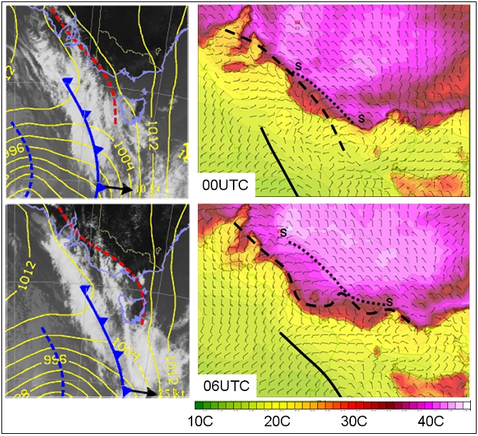
Mean sea level pressure and main synoptic features, trough corresponding to Type 2 cold front in red. superimposed upon the infrared satellite image for the shallow cold front of 17th January 2014 (LHS), Surface wind and temperatures (RHS) with the location of the cold front (bold black line), the pre-frontal trough (dashed line) and the wind change corresponding to the head of the Type 2 cold front (dotted line "s-s").
MSLP, Potential Temperature, Winds and Vertical Velocity
|
|
Figure 22: Parameters: MSLP, Potential Temperature, Winds and Vertical Velocity Left image courtesy BOM, centre and right images from Engel et al. 2012
|
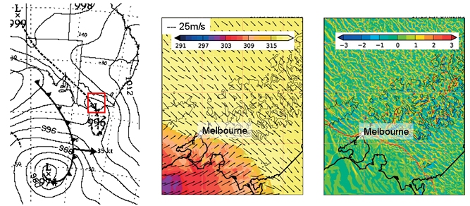
Useful Type 2 front parameters. (LHS) Mean sea level pressure 06 UTC 7th Feb, (CENTER) 500 meter potential temperature (K) and horizontal winds (m/s), (RHS) vertical velocity (m/s) 0615 UTC 7th February
MSLP, Virtual Potential Temperature, Relative Vorticity, Horizontal Winds
|
|
Figure 23: Parameters: MSLP, Virtual Potential Temperature, Relative Vorticity, Horizontal Winds Image from Thomsen et al. 2009
|
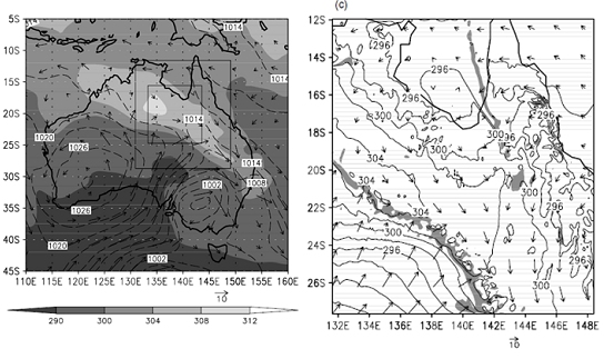
Useful parameters for the Central Australian front. (LHS) ECMWF analyses of MSLP, horizontal wind vectors and virtual potential temperature at 850 hPa at 10EST on 10 Sept. (RHS) potential temperature, horizontal wind vectors and relative vorticity on the omega=0.955 surface at 03 EST on 10 September. The shaded region marks the regions where the magnitude of the cyclonic relative vorticity exceeds 7.5 x 10⁻⁵ s-1 and this clearly shows the position of the front.
SLP, Winds, Vorticity
|
|
Figure 24: Parameters: SLP, Winds, Vorticity. Images from Reid 2000
|
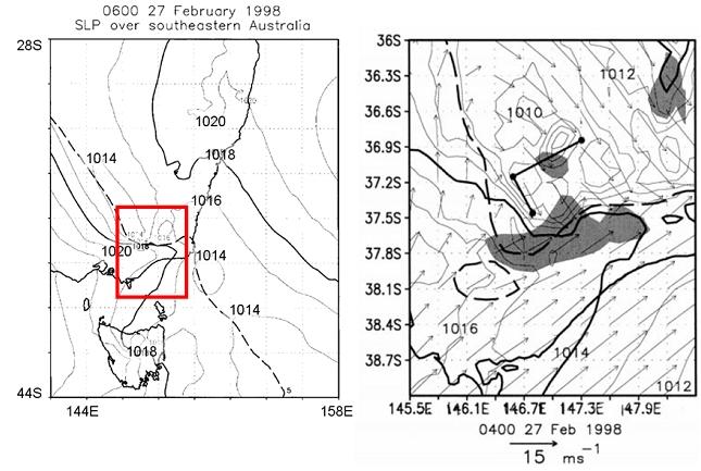
Useful parameters for the Southerly Buster. (LHS) sea level pressure (solid: 1018 hPa, bold), 5 m/s southerly wind contour is dashed, (RHS) seal level pressure (solid: 1014 hPa, bold), wind vectors with scale below, anticyclonic vorticity greater than 10-5 s-1 shaded.
Typical Appearance In Vertical Cross Sections
Here are some relevant NWP parameters that describe the vertical structure of Australian shallow cold fronts.
- Potential temperature contours give a good indication of the formation and strengthening of the front, as well as its depth thus verifying it as a shallow cold front. Wave features in the isentropes can reveal solitary waves travelling with or ahead of the front. In the case of Central Australian fronts the Potential Temperature can distinguish between a well mixed daytime boundary layer, the nocturnal regeneration of the Central Australian front as well as formation of the nocturnal inversion ahead of this.
- Equivalent potential temperature contours can distinguish between airmasses, permit the monitoring of airmasses that are being modified. Also permits analysis of atmospheric stability.
- Horizontal windspeed normal to the cross section. This reveals wind changes associated with the front, defining the front better. It also shows the development of the nocturnal jet in the case of the Central Australian front.
- Vertical velocity. Important in defining the location of the front, also the strength of the frontal updraft.
- Vorticity shows subtle features associated with the shallow cold fronts including pre-frontal solitons etc. Anticyclonic vorticity is important in defining the building of the ridge of high pressure accompanying the development of the Southerly Buster
- The Frontogenesis function, the Eddy exchange coefficient of momentum and convergence / deformation have also been used (not described here)
Note that station or model soundings are also very useful in identifying shallow cold fronts.
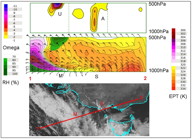
Equivalent Potential Temperature, Omega, Relative Humidity, Wind
|
|
Figure 25: Parameters: Equivalent Potential Temperature, Omega, Relative Humidity, Wind. Images courtesy JMA and BOM
|
Cross-section across the shallow cold front of 17th January 2014 along the axis 1-2 showing variations in vertical motion (omega) in the top diagram, equivalent potential temperature, relative humidity and wind direction and strength in the middle diagram and the corresponding visible satellite image. S shows the nose of the shallow cold front, M is the head of the Southern Ocean front. A is the vertical motion associated with the shallow cold front and U with the Southern Ocean front.
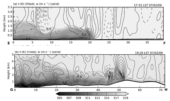
Potential Temperature, Vertical Motion
|
|
Figure 26: Parameters: Potential Temperature, Vertical Motion Images from Engel et al. 2012
|
Cross section of potential temperature (shaded) and vertical motion of the Black Saturday (Type 2) shallow cold front as it makes landfall at Melbourne and as it interacts with the topography of the Great Dividing Range.
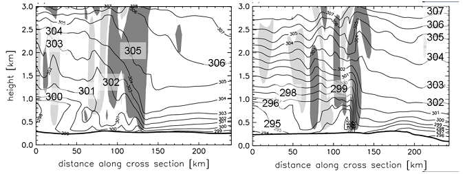
Potential Temperature, Vertical Wind Speeds
|
|
Figure 27: Potential Temperature, Vertical Wind Speeds Images from Thomsen et al. 2009
|
Central Australian Fronts. (LHS) 06EST on 10 September 1991 (RHS) 06EST on 17 September 1991. Potential temperature (K) and vertical wind speeds greater than 10cm/s (dark), and less than -10cm/s (light). The fronts are moving from left to right with the strongest upward motion at the head of the front. Note that the Central Australian Front of the 10 September 1991 (LHS) has amplitude ordered solitary waves travelling with the front.
Weather Events
Significant weather events are associated with all of the fronts and these are shown in the schematic diagrams and summarised in the table below. A challenging and significant forecasting problem concerns the tracking of the fronts, which is a particular issue for Type 2 and Central Australian fronts. There is often an abrupt change in frontal location in the transition from weakening Southern Ocean front to the strengthening Type 2 front. The Central Australian front is difficult to locate during the daytime but becomes very well defined at night.
|
|
Figure 28: Schematic of weather associated with Central Australian Fronts.
|
|
|
Figure 29: Schematic of weather associated with a Southerly Buster.
|
|
|
Figure 30: Schematic of weather associated with a Type 2 cold front.
|
| Parameter | Description |
|---|---|
| Precipitation |
|
| Temperature |
|
| Wind (incl. gusts) |
|
| Visibility |
|
|
|
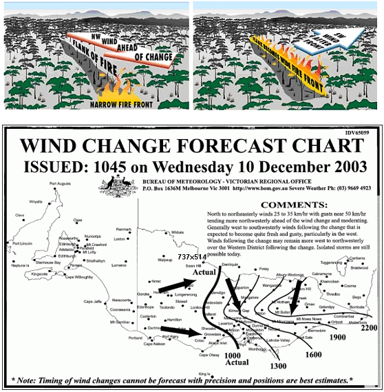
Figure 31: An example of one of the forecasting issues associated with Australian summertime shallow cold fronts. LHS - the changes in the geometry of the bushfire with the passage of the shallow cold front. RHS - the Wind Change Fire Chart produced by the Australian Bureau of Meteorology.
|
References
- American Meteorological Society Glossary. Internet reference http://glossary.ametsoc.org/wiki/Main_Page accessed January 2014
- Australian Bureau of Meteorology. "The Big Bust - Southerly Busters Explained!" http://www.bom.gov.au/social/2011/10/southerly-busters/
- Baines, P.G. 1990 "What's interesting and different about Australian meteorology" Aust. Met. Mag. 38 (1990) pp. 123-141
- Berry G., Reeder M.J., Jakob C. 2011 "A global climatology of atmospheric fronts" Geophysical Research Letters, Vol.38.
- Colquhoun J.R, Shepherd D.J., Coulman C.E., Smith R.K., McInnes K. 1985 "The Southerly Burster of South Eastern Australia: An Orographically Forced Cold Front" Monthly Weather Review Volume 113, pp 2090 - 2107
- Deslandes R. 2002 "Identifying dry fronts using satellite imagery" presentation at the Australia-Pacific Satellite Applications Training Seminar (APSATS). Australian Bureau of Meteorology.
- Deslandes R, Reeder M.J, Mills G. 1999. "Synoptic analyses of a subtropical cold front observed during the 1991 Central Australian Fronts Experiment". Aust. Meteorol. Mag. 48: 87 - 110.
- Engel, C. B., T. P. Lane, M. J. Reeder and M. Rezney. 2013. The meteorology of Black Saturday. Quart. J. Roy. Meteor. Soc., 139, 585 - 599. doi:10.1002/qj.1986.
- Garratt J.R. 1988 "Summertime Cold Fronts in Southeast Australia - Behaviour and Low-Level Structure of Main Frontal Types" Monthly Weather Review Vol 116, pp.636-649
- McInnes K. L., 1993: Australian southerly busters. Part III: The physical mechanism and synoptic conditions contributing to development. Mon. Wea. Rev., 121, 3261 - 3281
- Mills G.A. 2009 "Meteorological drivers of extreme bushfire events in southern Australia", CAWCR Modelling Workshop 2009. http://www.cawcr.gov.au/events/modelling_workshops/workshop_2009/papers/MILLS.pdf
- Mills G.A. 2010 "A westward propagating roll cloud and cool change on Tasmania's north coast" Australian Meteorological and Oceanographic Journal 60 pp. 237-247.
- Muir, L. C., and M. J. Reeder. 2010. Idealised modelling of landfalling cold fronts.Quart. J. Roy. Meteor. Soc., 136, 2147–2161.
- Physick W.I. 1988 "Mesoscale modelling of a cold-front and its interaction with a diurnally heated land mass". J.Atmos.Sci. 45: 3169-3187
- Reeder M.J. 1986 "The interaction of a surface cold front with a prefrontal thermodynamically well mixed boundary layer" Austral. Meteorol. Mag. 34: 137-148
- Reeder, M.J., Smith, R.K. 1992, "Australian spring and summer cold fronts" Australian Meteorological Magazine. Vol. 41, December 1992. pp. 101-124
- Reeder, M.J., Smith, R.K. 1998: Mesoscale meteorology in the Southern Hemisphere. Chapter 5 of Meteorology of the Southern Hemisphere. Ed. D. J. Karoly and D. Vincent. American Meteorological Society Monograph, No. 49, 201-241.
- Reid, H.J. 2000, "Regeneration of the Southerly Buster of Southeast Australia". Weather and Forecasting Vol.15, pp432-446
- Ryan, B.F., Wilson, K.J. Garratt J.R. and Smith R.K 1985. "Cold Fronts Research Programme: Progress, Future Plans and Research Directions". Bull. Am. Met. Soc., Vol. 66, No.9 pp. 1116 - 1122
- Tepper, M. 1950 "A proposed mechanism of squall lines: The pressure jump line". J. Met., 7, pp. 21-29
- Thomsen G.L., Reeder M.J., Smith R.K. 2009. "The diurnal evolution of cold fronts in the Australian subtropics" Q.J.R. Meteorol. Soc. 135: pp.395-411.