Cloud Structure In Satellite Images
The shallow cold fronts propagate within environments that generally have very limited amounts of atmospheric moisture. Type 2 fronts and Southerly Busters are best observed in the visible images due to shallow nature of front and the associated low-level cloud. The Central Australian Front is commonly tracked at night using enhanced infrared imagery. Progression of the fronts over the maritime regions may be monitored using satellite microwave scatterometer data.
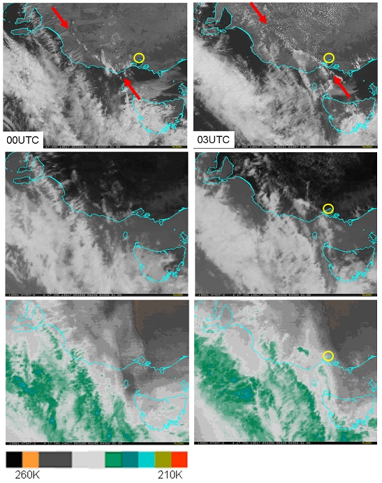
The Type 2 shallow cold front which crossed western parts of Victoria, Australia on the 17 January 2014 at times 00UTC and 03UTC is annotated by red arrows and shown in the visible (top), infrared (middle) and enhanced water vapour imagery (bottom). Clearly the visible image is the best for viewing this feature, though the infrared image may be useful at night. The location of the city of Melbourne is shown as a yellow circle.
Schematic diagrams of cloud signatures of three EXCY episodes are shown below.
|
|
|
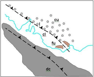
Figure 2 & 3: Schematic and satellite image of the cloud signatures and other features of a Type 2 front. Courtesy of Japan Meteorological Agency (JMA) and Australian Bureau of Meteorology (BOM)
|
|
Schematic of the cloud signatures and other features of a Type 2 front that can be detected in satellite imagery.
| Dc | deep cloud associated with the weakening Southern Ocean front (visible, infrared, water vapour) |
| Fu | smoke plumes from bushfires that change direction as the Type 2 front crosses the location (visible, sometimes infrared). |
| Cu | cumulus cloud can sometimes be seen upstream of this front (visible, infrared) |
| L | a line of cumulus cloud can sometimes be seen associated with this front (visible, infrared) |
| Cl | mostly clear of cloud on land behind the front |
|
|
|
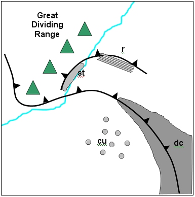
Figure 4: Schematic of the cloud signatures of a Southerly Buster.
|
Schematic of the cloud signatures of a Southerly Buster that can be detected in satellite imagery.
| Dc | deeper cloud associated with the cold front (visible, infrared, water vapour) |
| St | low cloud banking up against the escarpment of the range behind the Buster (visible, sometimes infrared). |
| r | roll clouds may be associated with the buster. (visible, sometimes infrared) |
| Cu | speckled cumulus cloud behind the cold front (visible, infrared) |
|
|
|
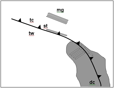
Figure 5: Schematic of the cloud signatures and other features of a Central Australian Front that can be detected in satellite data.
|
Schematic of the cloud signatures and other features of a Central Australian Front that can be detected in satellite data.
| Tc | cooler temperatures at night ahead of the front (infrared) |
| Tw | warmer temperatures at night behind the front (infrared) |
| Mg | morning glory cloudlines ahead of the front and near the Gulf of Carpentaria (visible) |
| St | low cloud associated with the front during the day (visible) |
| Dc | deeper cloud associated with the original Southern Ocean Cold Front over eastern Australia (visible, infrared, water vapour) |
Type 2 front in various satellite channels/products
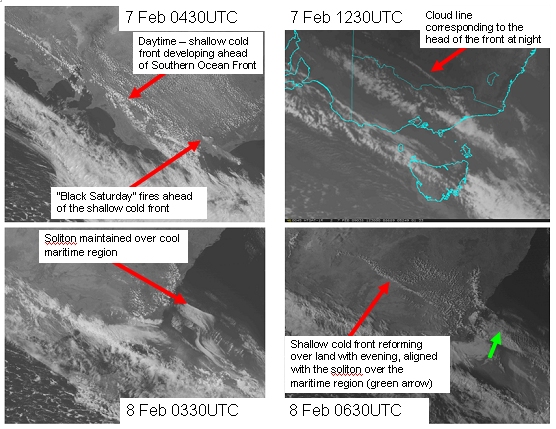
The evolution of the Type 2 front corresponding to the “Black Saturday Bushfire” event is shown in visible and infrared imagery below. A line of cumulus marks the region of surface convergence and frontogenesis. The broad cloudband corresponding to the Southern Ocean front is seen to the southwest. The eastward progression of the shallow front can thus be monitored using visible imagery during the day and infrared imagery during the night, provided there is sufficient low level moisture available to maintain the cloud line along the nose of the front. In the 0430 UTC image shallow cumulus cloud streets may be observed to develop in the warm northwesterly airstream ahead of the front. Note that the front cannot be detected over land at 0330UTC on the 8th February presumably due to the mixing of dry air through the deep daytime continental boundary layer. However, its progress may be followed over the adjacent maritime region as low level stratiform cloud associated with the passage of a solitary wavetrain.
Note that there is an absence of cloud in the cool and stable post-frontal region.
|
|
|
Figure 6: Evolution of a Type 2 shallow cold front, Black Saturday fire event, 7-8 February 2009 in visible and infrared (1230UTC) MTSAT-1R imagery. Images courtesy JMA and BOM
|
Southerly Buster
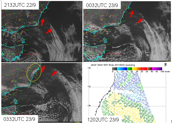
As shown in the figure below, the location of the parent cold front to the Southerly Buster can be clearly seen in satellite imagery as a sharply defined cloud line embedded within the frontal band and located in the Tasman Sea to the east. Closer to the east coast of Australia the dry continental westerly offshore flow is suppressing cloud formation. However, a wave train of solitary waves or a single roll cloud may sometimes be seen at the head of the Buster in the visible image though this is not so clear in the corresponding infrared image.
In the 0332UTC image the passage of the Buster can also be detected by the stratus cloud banking up against the ranges in the cold air behind the change as shown within the yellow circle. Microwave scatterometer data such as ASCAT and WindSAT is also useful in monitoring the progress of the Buster, however this polar orbiting satellite data has limited temporal frequency.
|
|
|
Figure 7: Cloud features associated with the Southerly Buster of 23 September 2011, MTSAT-1R visible imagery and ASCAT scatterometer winds. Red arrows indicate the leading edge of the Buster. The low cloud banking up against the escarpment behind the passage of the Buster is located within the yellow ellipse. Images courtesy JMA and BOM, bottom right image courtesy NOAA/STAR
|
Central Australian fronts
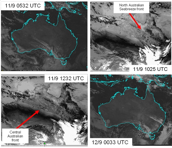
Central Australian fronts are best detected during the night when the fronts have the strongest intensity and the most pronounced signal in the infared channel. Inspection of an animated loop of this imagery defines the front as dividing the cooler nocturnal inversion ahead from the warmer turbulent boundary layer behind the front. “Southern Morning Glories” travelling ahead of the front may be detected using the visible channel during the daytime.
|
|
|
Figure 8: Cloud features associated with the Southerly Buster of 23 September 2011, MTSAT-1R visible imagery and ASCAT scatterometer winds. Red arrows indicate the leading edge of the Buster. The low cloud banking up against the escarpment behind the passage of the Buster is located within the yellow ellipse. Images courtesy JMA and BOM, bottom right image courtesy NOAA/STAR
|
In the visible daytime images shown above it can be seen that the band of cloud associated with the higher latitude front may persist over southern and eastern parts of the continent as the Central Australian front moves northwards. The progression of this can be followed in the visible and infrared images. Cloud streets oriented parallel to the direction of boundary layer wind shear can be seen in the visible images shown below.
|
|
|
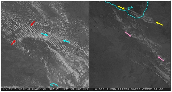
Figure 9: Cloud features associated with Central Australian front event of the 16th September 1991. Images courtesy JMA and BOM
|
Left-hand side: pre and post frontal cloud streets, blue arrows show pre-frontal cloud streets oriented in a northwesterly direction, red arrows indicate post frontal cloud streets oriented in a southwesterly direction. Right-hand side: the cloud features on the following morning. Yellow arrows annotate the solitons (Morning Glory), pink arrows indicate the approximate position of the surface front. GMS-5 visible imagery.
|
|
|
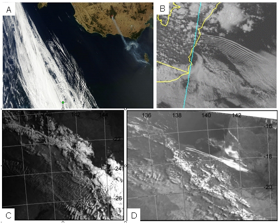
Figure 10: Solitary waves and wave-trains associated with different cold fronts. Top left image courtesy NASA/GSFC Rapid Response, top right image courtesy JMA and BOM, bottom images from Thomsen et al. 2009
|
Solitary waves and wave-trains associated with different cold fronts:
A: ahead of a Southern Ocean front, 18 February 2013 0030UTC Terra MODIS image.
B: associated with a Southerly Buster, 7 January 2009 MTSAT-1R visible image.
C: associated with a Central Australian front, propagating with the front 10 September 1991 0818EST NOAA-12 AVHRR image.
D: associated with a Central Australian front, propagating ahead of the front as a 'Morning Glory' 17 September 1991 0730EST NOAA-12 AVHRR image.