Chapter IX:LST Applications
Table of Contents
LST as input for Evapotranspiration Models
The present chapter covers some applications where LST data is currently being used.
Actual Evapotranspiration can be estimated by satellite by using an energy balance method. WACMOS-ET is an ESA project which derives ET estimations from a group of ET models driven by satellite-based inputs. One of these inputs LST, has been computed for a three-year period (2005-2007) for a set of instruments (AATSR (EnviSat), SEVIRI (MSG), MTSAT and GOES-E) using algorithms and inputs as common as possible among all instruments, thus providing a consistent, nearly global dataset for both GEO and LEO platforms.

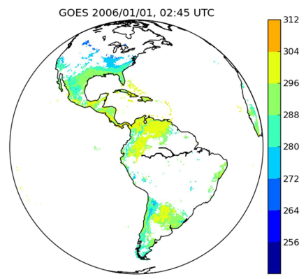
Fig. 34: Example maps of LST products used in the ESA WACMOS-ET project. Source: The WACMOS-ET Land Surface Temperature dataset. Poster presented at the 6th LSA SAF Workshop: http://landsaf.ipma.pt/workshops.jsp?seltab=1&starttab=0
Features in maps
LST maps allow identifying surface features such as mountains, cities and inland water bodies, as shown in Fig. 35. Some features are highlighted in this LST map from Europe on 15 August 2009 at 00 UTC; mountains are indicated with white circles, lakes/rivers in green and the city of Paris in red.
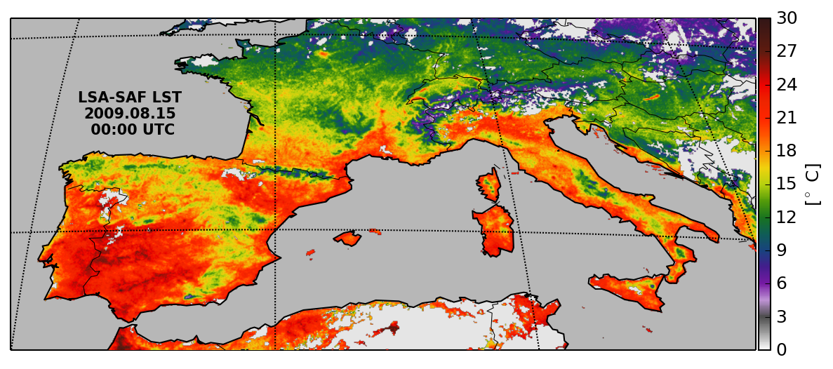
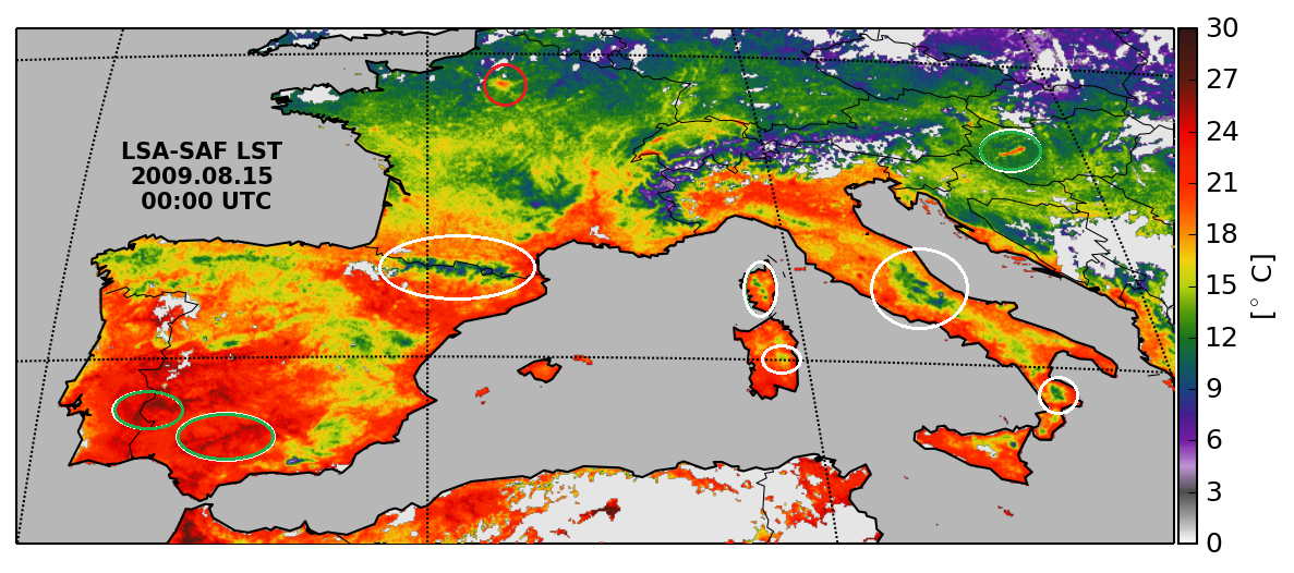
Fig. 35: LST map from Europe on 15 August 2009 at 00 UTC. Obtained from the LSA SAF.
The Nile Delta is clearly distinguishable in the maps of maximum LST (LSA SAF) 10 days composite for September 2014 (Figure 35). Also, there is a green area over the arid region of Negev desert (South of Berseba) (LST~47°C) in Israel, contrasting with the higher temperatures (~55°C) observed over the deserts of Egypt to the west. There is little rain in this area in July and August and so the desert should be dry everywhere. Yet, for the past several years, the Israeli government has invested much in transforming the northern Negev (the desert covers around 60% of the country's land area) into an agricultural land, partially irrigated. The maps of maximum LST in parts of Egypt and Israel from September 2014 are shown in Figure 35. During the first ten days the temperatures in southern Israel are moderate due to irrigation. After that rain starts to fall and the differences between Israel and Egypt diminish.
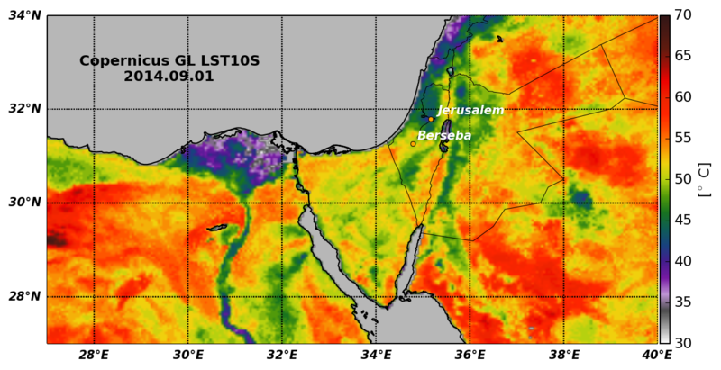
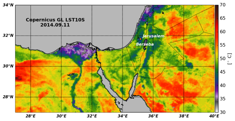
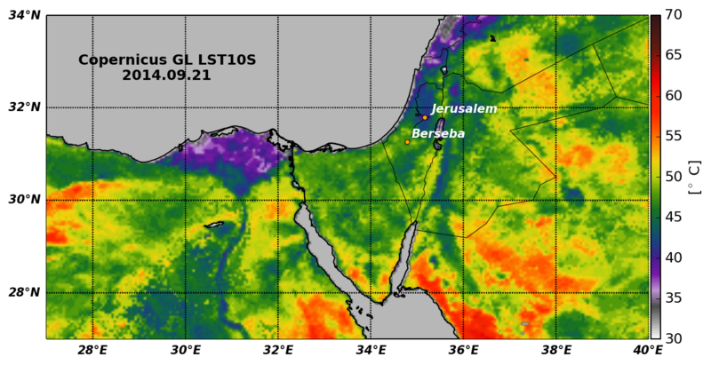
Fig. 36: Maximum LST 10 days composites for September 2014 (LST LSA SAF product) over Egypt and Israel.
Urban Heat Islands
The Urban Heat Islands effect has been a topic of increasing concern over the last decades. By replacing plants (which cool their surroundings by evaporating water) with impervious surfaces, heat is trapped, leading to city centers warmer than surrounding rural areas by several degrees. A variety of factors are involved in the phenomenon, but overall bigger cities tend to have stronger heat-trapping capacities than smaller ones and cities surrounded by forest have more pronounced heat islands than cities in arid environments. Figure 36 shows how big cities are easily identified in the LST map from 26 May 2012 at 13:00 UTC in the UK.
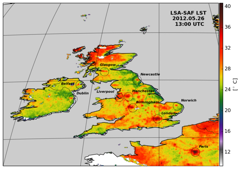
Fig. 37: Identification of large cities in the UK and Ireland using LST map product from LSA SAF on the 26 May 2012 at 13:00 UTC.
The UHI effect can be particularly dangerous during heat waves. This has actually been causing an increasing number of casualties among the elderly - particularly in southern Europe (http://www.urbanheatisland.info/). In light of this, ESA has funded a project (2008-2011) in which UHI trends over 10 European cities (Athens, Bari, Brussels, Budapest, Lisbon, London, Madrid, Paris, Seville, Thessaloniki) were analyzed over a period of ten years , using a multi-sensor approach in order to make the best use of all satellite missions that carry TIR sensors (SEVIRI, AVHRR, AATSR, MODIS, LANDSAT, ASTER). The purpose was to aid decision and policy makers in mitigating the effects of UHIs through appropriate alert systems and, in terms of reducing risk, through improved urban planning (http://www.urbanheatisland.info/).
Climate Change
A long-term trend in surface temperature is a key indicator of climate change. One limitation of satellite data for climate change studies is data longevity. Nevertheless, this can be partially minimized by the use of data from polar orbiters. LST from AVHRR has been available for nearly 20 years (since NOAA 14).
As mentioned before, NASA has been providing maps of average monthly land surface temperature in degrees Celsius as measured by MODIS on NASA's Terra satellite since the year 2000.
For climate change studies, analyzing anomalies is the best way to find out the trends. NASA also provides maps that compare daytime land surface temperatures in a particular day, week or month compared to the average conditions during a given period between 2001-2010. An example is shown in Figure 37, for August 2015, showing positive anomalies over central Europe.
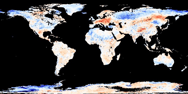
Fig. 38: LST from the Terra satellite's MODIS instrument for August 2015 as provided by NASA. Places that are warmer than average are red, places that were near-normal are white, and places that are cooler than average are blue. Black means there is no data.
Source: http://neo.sci.gsfc.nasa.gov/view.php?datasetId=MOD_LSTAD_M&year=2015 (Images by Jesse Allen, NASA's Earth Observatory using data courtesy of the MODIS Land Group).
Long time series from geostationary satellites
Although they provide long data series, sensors onboard polar orbiter satellites such as AVHRR and MODIS, cannot provide information about the LST diurnal cycle, with only two passages per day.
The data from the sensors onboard the Meteosat First and Second Generation provide a daily LST cycle for over 30 years with 1 h temporal frequency and 5 km spatial resolution, provided that consistency between data from all Meteosat satellites is ensured. LSA SAF and CM SAF have developed a consistent single channel LST retrieval algorithm for all Meteosat sensors (since MVIRI on Meteosat 2-7 was equipped with a single thermal channel, a mono-channel algorithm is used). LST Meteosat Climate Data Record (CDR) will be released in 2017. For more information see Anke Tetzlaff's report from the 6th LSA SAF Workshop: 'Suitability of Meteosat satellite data for climatological LST retrieval'.
Extreme events monitoring
Heat Waves
Heat waves are natural hazards that cause deaths and financial loss due to crop deficit and forest fires. LST maps can help monitor such events and assess the spatial extent of the affected areas.
2003 Heat Wave - Western Europe
Figure 38 shows the heatwave that hit Europe in July 2003. The image corresponds to LST anomaly computed in July 2003 compared to July 2001, as observed by MODIS on NASA's Terra satellite.
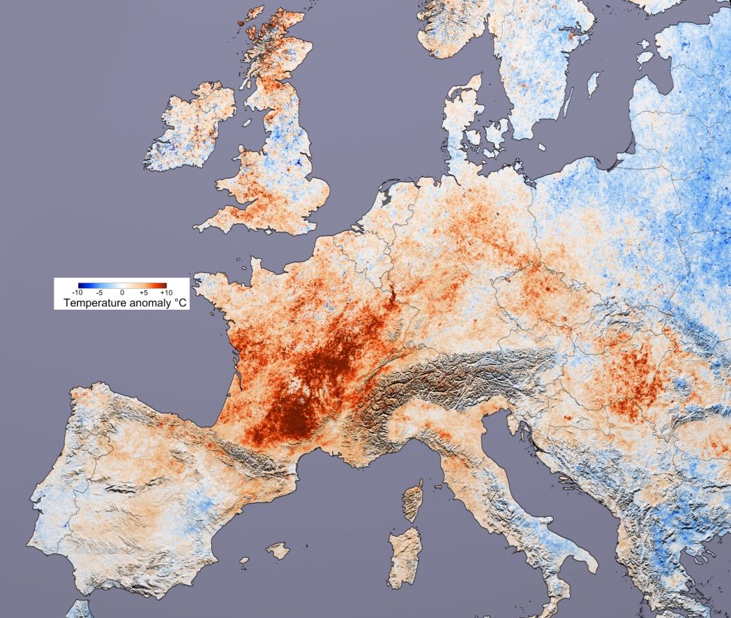
Fig. 39: 2003 heat wave temperature variations in Europe relative to July 2001. This image shows the differences in day time land surface temperatures collected by MODIS on NASA's Terra satellite. "Compared to July 2001, temperatures in July 2003 were sizzling."
http://earthobservatory.nasa.gov/IOTD/view.php?id=3714
2007 Heat Wave - Eastern Europe
The 2007 European heat wave affected most of southern Europe and the Balkans as well as Turkey. During July, Greece, Italy, Bulgaria, Romania, the Republic of Macedonia, and Serbia were the most affected countries. There were widespread fires in the region as a result of the phenomenon.
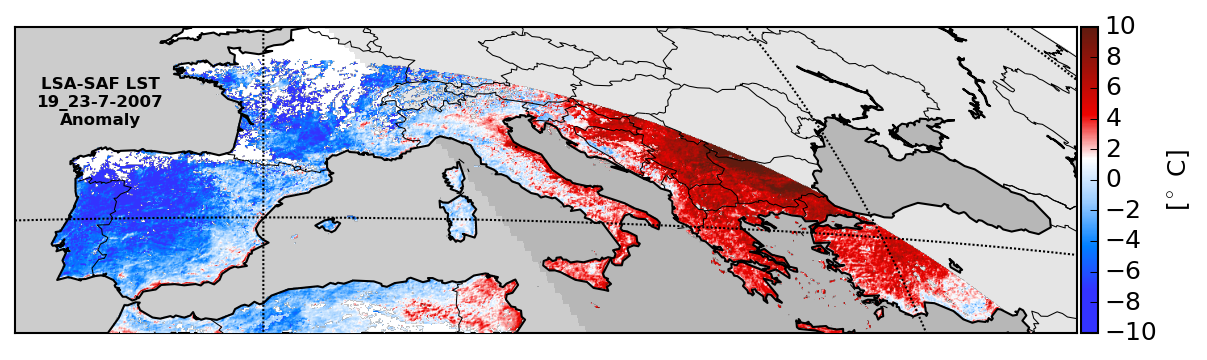
Fig. 40: On July 2007 a heat wave hit central Europe affecting especially Italy, Bulgaria and Romania.
2010 Heat wave - Central, Eastern and Southwestern Europe
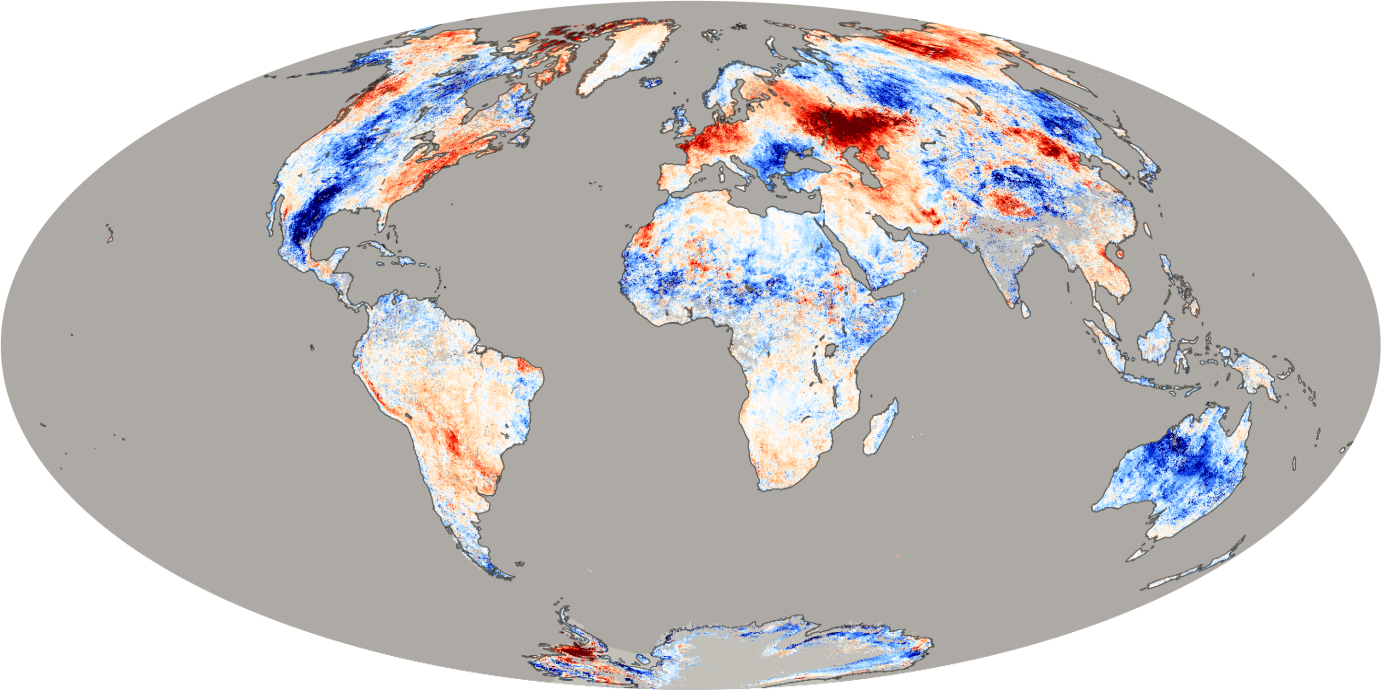
Fig. 41: LST anomalies as depicted by MODIS onboard the Terra satellite from 4 through 11 July 2010, compared to temperatures for the same dates from 2000 to 2008. Oceans, lakes, and areas with insufficient data (usually because of persistent clouds) appear in gray.
Source:
http://eoimages.gsfc.nasa.gov/images/imagerecords/44000/44664/globallsta_tmo_2010185_lrg.png
Fig. 42 shows the LSA SAF LST product is consistent with MODIS while detecting this temperature anomaly.
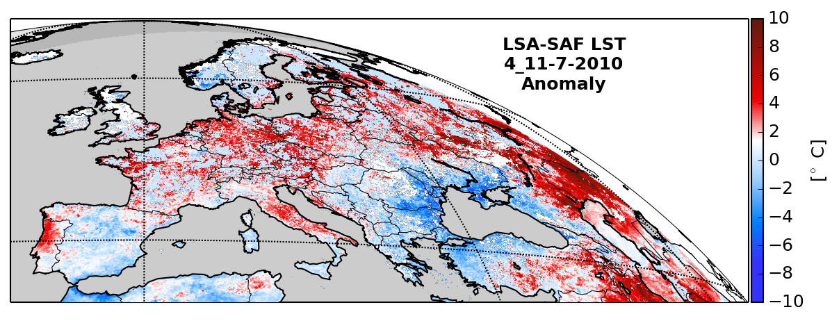
Fig. 42: LSA SAF LST product anomaly from 4 through 11 July 2010: positive values are observed in northern Portugal and central Europe. A positive anomaly is also observed over countries around the Caspian Sea.
2013 Heat Wave in UK and Ireland
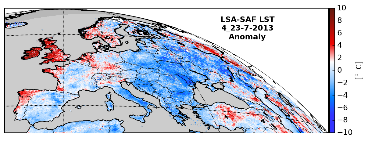
Fig. 43: LST anomaly as depicted by the LSA SAF LST product from 1 through 23 July 2013 over the UK and Ireland, compared to July averages between 2009-2012.
The 2013 heat wave in the United Kingdom and Ireland was a period of unusually hot weather primarily in July 2013. A prolonged high pressure system over Britain and Ireland caused higher than average temperatures for 19 consecutive days in July, reaching 33.5°C at Heathrow and Northolt (Wikipedia).
Cold periods
The East Coast of the USA has been experiencing cold periods from 2012 to 2015. February 2015 saw particularly low temperatures. This pattern is well documented by the Land Surface Temperature (LST) Product as shown in the maps of its median over each dekad or ten-day period of February. The most extreme LST values are observed during the 2nd dekad of February 2015.
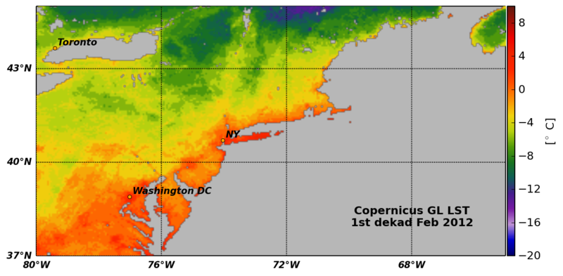
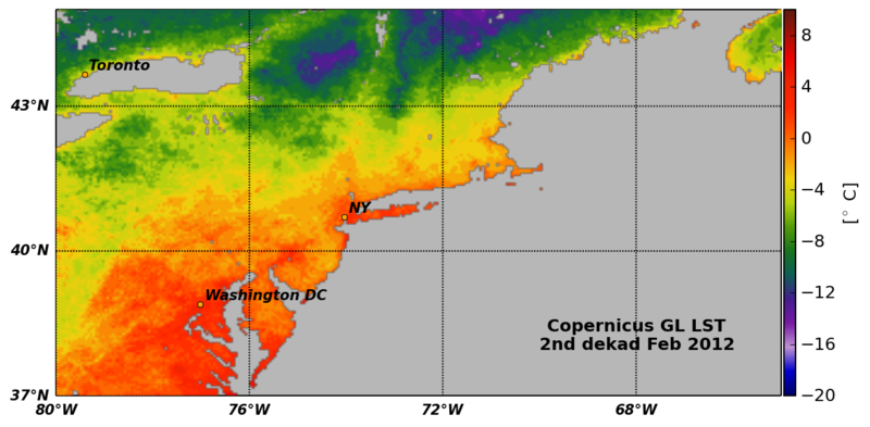
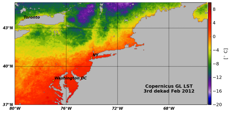
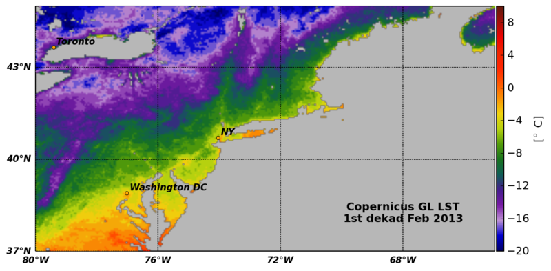
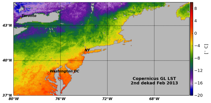
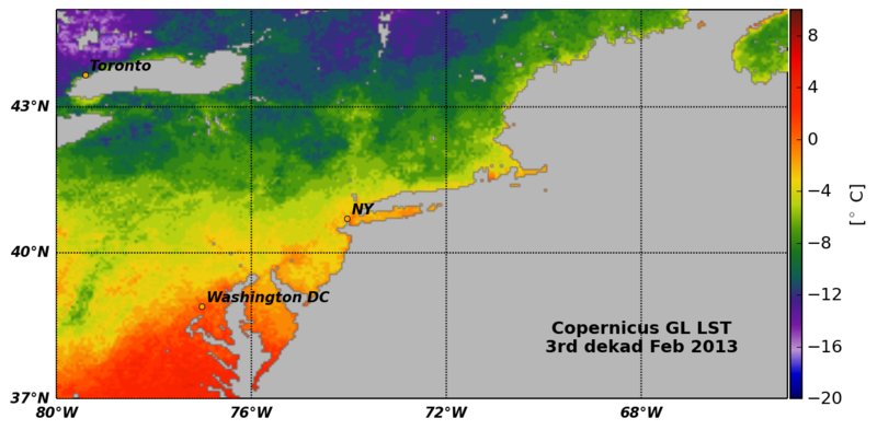
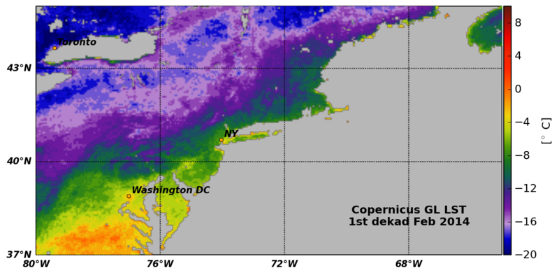
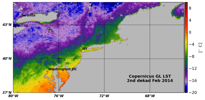
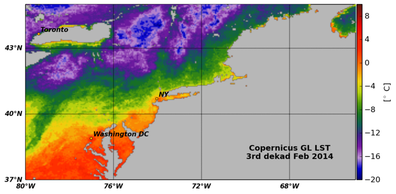
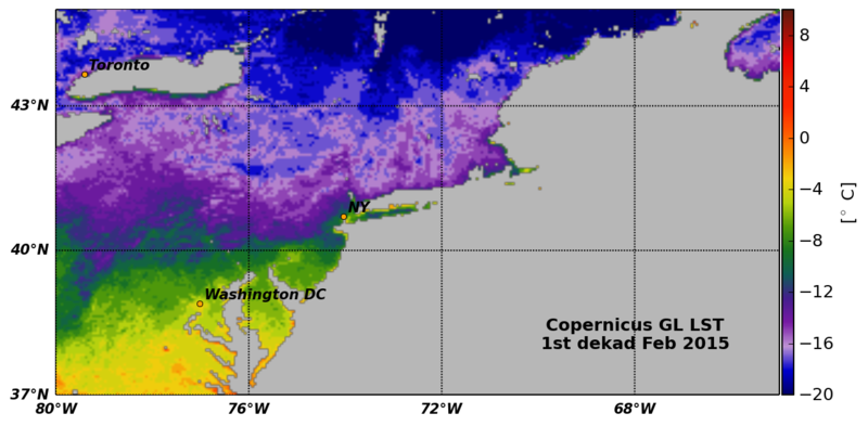
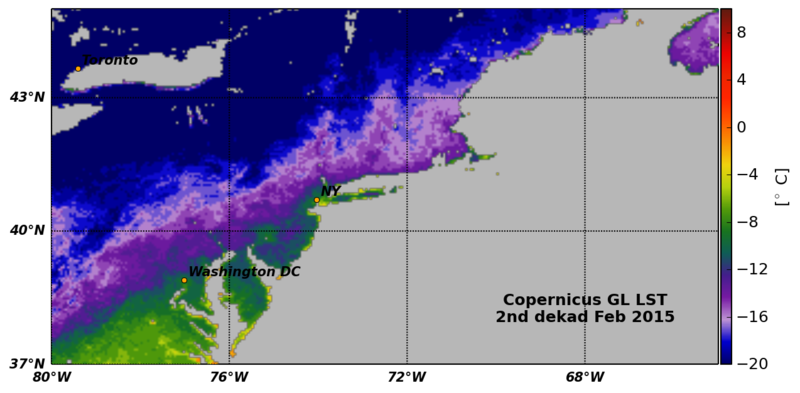
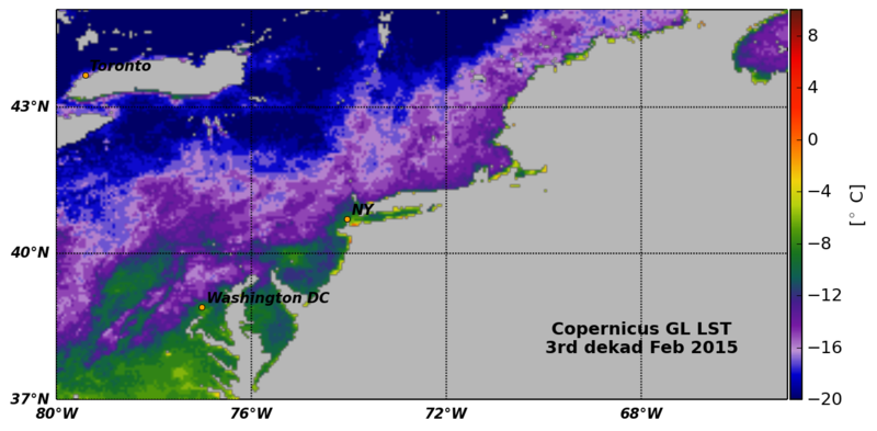
Fig. 44: LSA SAF Surface Temperature (LST) median values over each dekad of February 2012 to 2015. The most extreme LST values were recorded during the 2nd dekad of February 2015.
Modelling studies
Assimilation of LST has the potential to improve land surface model parameters.
The next figure, extracted from http://lst.nilu.no/language/en-US/ApplicationsofLST.aspx shows the influence that assimilation of LST has on the state of the modelled soil moisture. As shown, there is a better agreement between soil moisture observations (blue line) and modelled soil moisture with assimilated LST (red line) than between the observations and data resulting from open loop modeling (green line).
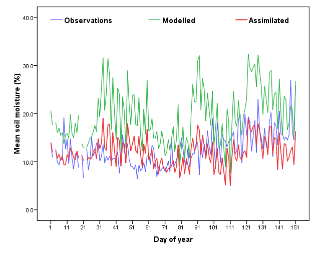
Fig. 45: This image shows a time series of open loop modeling (green) vs. model run following LST data assimilation (red) for mean daily soil moisture values over a region of West Africa from 1 January - 31 May 2007. ERS scatterometer surface soil moisture observations are plotted for comparison (Ghent et al., 2010).
Burned area mapping
Burned areas tend to have higher surface temperatures than surrounding non-affected vegetation shortly after a fire. This is explained by the fact that charcoal and ash absorb more energy than vegetation and also because there is no cooling from the vegetation formerly covering the burned area and the loss of soil moisture. LST data from sensors onboard polar platforms for burned area mapping have been used in several studies.
This increase in LST over burned areas has been used in algorithms that combine remote-sensed information on the near- and thermal infrared regions to distinguish burned areas. Figure 45 presents results for Portugal on 4 August 2003, obtained using fuzzy logic methods. This approach utilizes information from near- and thermal infrared channels from the AVHRR sensor onboard NOAA satellites, and computes the probability (on a scale from 0 to 1) that a given pixel is within a burned area.
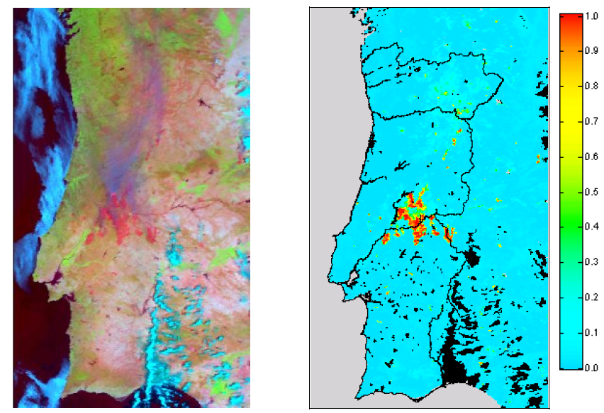
Fig. 46: The summer of 2003 was characterized by very warm and dry conditions in Europe, especially in the west. In particular, it was the short-lived heatwave that occurred in the first fortnight of August that was responsible for the worst fire occurrences ever recorded in continental Portugal. According to official data, the burned area reached a total amount of 453,097 ha, 304,182 ha of which (i.e. 66% of the total) were recorded in the first two weeks of August, and 91,439 ha (i.e. 22% of the total) were recorded on 4 August. It is worth emphasizing that wildfires in August were responsible for the death of 21 people and an estimated loss of 15.5 million euros. The left panel represents an RGB (channel 4 - thermal infrared, channel 2 - near-infrared, channel 1 - red) of an AVHRR/NOAA image on 4 August 2003. The right panel represents the output of the neuro-fuzzy system (Calado et al., 2005) that utilizes information from the near- and thermal infrared region to produce a probability from 0 (no possibility that a pixel is burned) to 1 (full possibility that a pixel is burned).
Another important variable related to fires is the Fuel Moisture Content (FMC) of vegetation, since it is a driving factor of wildfire susceptibility and wildfire behavior. FMC of a sample is determined by dividing the difference between the wet and dry weights by dry weight of that sample. Potential improvements in live FMC estimations have been gained by incorporating information about satellite-derived surface temperature, as this variable would be expected to increase in drier plants due to decreased evapotranspiration.