Product Tutorial on Land Surface Temperature (LST)

Methods to retrieve LST from satellite infrared measurements

From the previous chapter we can conclude that the major difficulty when measuring LST is the uncertainty about land surface emissivity. The different algorithms that have been proposed to solve the RTE can be divided in two distinct categories:

1. Land Surface Emissivities (LSEs) are assumed to be known beforehand
2. LSEs are not known in advance.

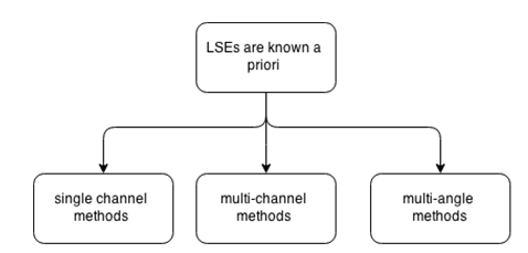
Fig. 10: Methods to estimate LST assuming surface emissivity is known in advance are classified in single channel, multi-channel and multi-angle methods.

If the emissivity is assumed to be known in advance, the RTE equation is solved in order to retrieve the LST. There are three different ways of solving these equations: single channel, multi-channel and multi-angle methods (Figure 10).

If no emissivity value is known in advance, the purpose of the algorithms is to solve the RTE for the two unknowns (LST and LSE). They can be classified as: stepwise retrieval methods, simultaneous retrieval of LST and LSE with known atmospheric information, and simultaneous retrieval of LST and LSE with unknown atmospheric information (Figure 11).

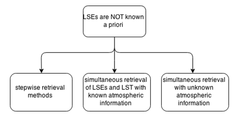
Fig. 11: Methods to estimate LST assuming surface emissivity is not known in advance: stepwise retrieval methods, simultaneous retrieval of LST and LSE with known atmospheric information, and simultaneous retrieval of LST and LSE with unknown atmospheric information.

The list of the advantages and drawbacks of these methods is quite extensive, and allow different accuracy values on LST retrievals. However, the choice of approach cannot be based solely on accuracy. The choice is governed by many factors, such as the availability and quality of the input data, the geographical area of application and allowed computation time. With this in mind, it should be mentioned that the methods that try to solve the LSE and LST simultaneously are computationally very heavy, and therefore not suitable for operational LST retrievals from a high temporal frequency satellite sensor, such as MSG's SEVIRI.

The next section provides a brief description of the different methods with examples of some reference algorithms. A detailed description of the methods and their assumptions, strengths and disadvantages, is found in Zhao-Liang Li et. al (2013).

 

Methods in which LSE is assumed to be known beforehand

1. Single channel methods

Methods that use one single satellite channel imply a simple inversion of the RTE. As mentioned earlier, the emissivity is assumed to be known, as is information about atmospheric composition. Currently atmospheric profiles from numerical prediction models forecasts and analyses are used as alternatives to radio soundings, which have a poor network density. Nevertheless, this has proven to produce large errors in LST retrieval (Chédin et al, 1985). On the other hand, the use of satellite sounders provides more accurate information. The problem is that there are not many instruments that have a thermal imager with sounders onboard, so satellite sounding data is not widely used. Single channel methods rely on the use of Radiative Transfer Models (RTMs) to simulate radiance at the TOA, so the method is also dependent on the accuracy of the RTM.

Figure 12 gives a schematic view of how single channel methods work: A dataset of brightness temperatures at the top of the atmosphere is simulated with a RTM using prescribed values of (LST, ε_λ) and atmospheric profiles. The obtained Lookup Tables (LUTs) are used to estimate LST, which corresponds to the sensor's BT.

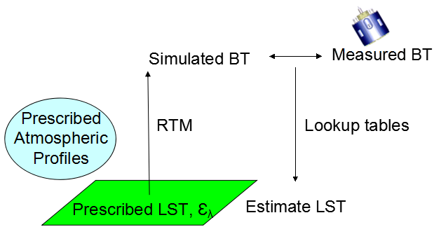
Fig. 12: A schematic of the general principle of single channel methods for LST retrieval.

2. Multi-channel methods

There are many sensors with more than one channel in the TIR suited to retrieving LST from satellites, such as those onboard MODIS, AVHRR, AATSR, MSG, GOES or Himawari. One of the most popular methods uses two channels centered at about 11 μm and 12.0 μm to account for the atmospheric effect. The difference in TOA radiances measured in channels near the TIR and with distinct atmospheric transmissivities gives an estimate of the atmospheric water vapor content. This technique, known as Split Windows (SW) was first proposed to estimate surface temperature over the ocean, where emissivity is homogeneous and can be assumed to be one with little detriment to LST calculations. For land surfaces, however, emissivity is highly variable spatially; it depends on the emissivity distribution within the pixel, the spectral range of measurement, and view angle. Yet, given the success of the SW technique, it has also seen widespread use over land. These algorithms were first developed for specific regions. Later, Wan and Dozier (1996) proposed an algorithm that can be applied to different regions of the globe and under distinct atmospheric conditions, named Generalized Split Windows (GSWs). Over the years several different GSW formulations have been proposed. These types of algorithms rely on the linearization of the RTE with respect to the temperature or the wavelength. A typical linear SW algorithm can be written as:

LST = a₀ + a₁T_i + a₂(T_i - T_j)  (eq.12)

where a_k (k=0, 1, and 2) are coefficients that depend primarily on the spectral response function of the two channels (i and j), the two channels' emissivities, water vapor content, and the satellite's viewing zenith angle (VZA).

There are also SW algorithms that rely on non-linear simplifications of the RTE, giving rise to formulations of the type:

LST = c₀ + c₁T₁ + c₂(T_i - T_j) + c₃(T_i - T_j)²  (eq.13)

where c_k (k=0-3) are coefficients pre-determined by regressing this equation with simulated satellite data values for a set of atmospheres and surface parameters.

Linear or non-linear multi-channel algorithms?

When more than 2 TIR channels are available, the LST can be estimated from a linear or non-linear combination of the TOA brightness temperatures in those channels using methods similar to the SW algorithms. As an example, the linear multi-channel formulation proposed by Sun and Pinker (2003) uses 3-channels (2 SW and the Middle Infrared (MIR) 3.9 μm) to estimate LST. It derives emissivity from the different surface types that cover a pixel and uses the MIR 3.9 μm channel to improve the atmospheric correction during night.

3. Multi-angle methods

Similarly to the SW, multi-angle methods rely on the estimation of atmospheric effects. It is assumed that in a given spectral channel an object is observed from different viewing angles, giving differing absorption values due to the distinct optical paths. It was primarily developed for the ATSR (Advanced Track Scanning Radiometer) onboard ERS -1, the first sensor operating in biangular mode, i.e., capable of providing 2 views of the same scene within about two minutes: at near-nadir (0°-22°) and at forward view under 55°.

LST retrieval with unknown LSEs

The methods described so far assume the surface emissivity to be known. However, accurate estimations of LSE at the pixel scale are hard to achieve beforehand. LSE is a characteristic of the surface, varying with vegetation cover, surface roughness and soil moisture, which are difficult to account for in laboratory-based measurements. Several methods have been developed to derive LSE from the emitted radiance measured by a sensor. Such methods will not be presented here, but just as an example, Fig. 13 shows emissivity maps as computed by the LSA SAF (In the LSA SAF the surface emissivities for each sensor channel are estimated as an average of bareground and vegetation emissivities within each pixel, weighted with the pixel Fraction of Vegetation Cover (FVC). The bareground/vegetation emissivities have been assigned to each class of a land cover map [Peres and DaCamara, 2005; Trigo et al., 2008], FVC is routinely retrieved by the LSA SAF) for SEVIRI channels 3.9, 8.7, 10.8 and 12.0 μm.

Fig. 13: Example of emissivity maps as computed by the LSA SAF SA SAF for SEVIRI channels 3.9, 8.7, 10.8 and 12.0 μm. The method uses the Vegetation Cover Method which considers the effective emissivity of each pixel as a weighted fraction of vegetation and bare ground components: ε_i = ε_ivegFVC + ε_iground(1 - FVC). FVC is the Fraction of Vegetation Cover, a product also computed in the LSA SAF.

1. Stepwise retrieval methods

In stepwise retrieval methods the LST and LSE are computed in two steps. First, the LSE is (semi-) empirically estimated from visible/near-infrared measurements or physically estimated from pairs of atmospherically corrected MIR and TIR radiances at ground level. In the following step the LST is computed using any of the retrieval methods described above: single, multichannel (SW) or multi-angle (dual-angle).

2. Simultaneous LST and LSE retrieval methods with known atmospheric information

In these methods LST and LSE are simultaneously retrieved from the atmospherically corrected brightness temperatures (atmospheric information is known so the TOA brightness temperatures are reduced to the ground level) either by reducing the number of unknowns (can be done with Principal Component Analysis techniques) or increasing the number of equations. These methods are further classified as multi-temporal and multi (hyper)-spectral retrieval methods. Methods in the first group assume emissivity is invariant over time. Consequently, considering 2 time slots t1 and t2 the problem we need to solve will have 2N equations (N-number of channels) for N+2 unknowns (LST^t1, LSE_ch1, LST^t2, LSE_ch2):

Channels (ch)	Time (t)
	1	2
1	LSTt1, LSEch1	LSTt2, LSEch1
2	LSTt1, LSEch2	LSTt2, LSEch2

From these methods two reference algorithms are the two-temperature (Watson, 1992) which considers a scene at two times in the diurnal cycle (optimally after midday and midnight), and the physics-based day/night (Wan & Li, 1997). In order to reduce the error of the atmospheric corrections, the latter method introduces two variables (air temperature at the surface level (Ta) and atmospheric water vapor (WV)) to modify the initial atmospheric profiles. With two measurements (day and night) in N channels, the number of unknowns is N+7 (N channel LSEs, 2 LSTs, 2 Ta, 2 WV, and 1 angular form factor in the MIR channels). Thus, to make the equations deterministic, the number of channels used in the retrieval must be equal to or greater than seven. Due to the high number of required spectral channels this method of solving LST cannot be used with the sensors onboard GOES; MSG, Metop. On the other hand, the MODIS (Moderate Resolution Imaging Spectroradiometer) with its seven TIR bands is suited to use this method for measuring surface temperatures.

https://cimss.ssec.wisc.edu/rss/bertinoro/source/text/15.pdf

Multi (hyper)-spectral retrieval methods use hyperspectral TIR data as input (that provides much more detailed information on the atmosphere and land surface) and rely on the intrinsic spectral behavior of the LSE.

3. Simultaneous LST and LSE retrieval methods with unknown atmospheric information

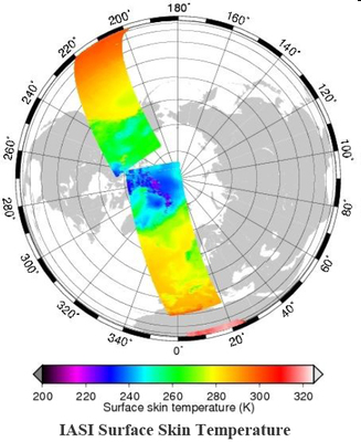
Fig. 14: LST estimated from the EUMETSAT Infrared Atmospheric Sounding Instrument (IASI) onboard the Metop satellite.

The simultaneous LST and LSE retrieval methods take advantage of the narrow bandwidth of the thousands of channels available from hyperspectral TIR sensors that improve the vertical resolution and allow atmospheric profiles and surface parameters (LST and LSEs) to be obtained more accurately (Chahine et al., 2001). An example of LST estimated from the Infrared Atmospheric Sounding Instrument onboard Metop is shown in Figure 14.