Creating Snow RGB images
The Snow RGB is composed of the VIS0.8, NIR1.6 and the 3.9 micrometer channel (IR3.9) data (Table 1). The measured values should be calibrated to calculate reflectivity (including also solar zenith angle correction). During daytime the IR3.9 radiance includes reflected solar contribution as well as emitted thermal radiation. In the Snow RGB we are interested only in the solar component. To create the snow RGB one has to calculate the solar component of the measured IR3.9 signal. The abbreviation IR3.9refl (in Table 1) indicates the reflectivity computed from the solar component of the measured IR3.9 radiation.
Table 1: 'Recipe' of the Snow RGB
| Colour beam | Channel | Range [%] | Gamma | |
|---|---|---|---|---|
| Red | NIR1.6 | 0 | 100 | 1.7 |
| Green | NIR1.6 | 0 | 70 | 1.7 |
| Blue | IR3.9refl | 0 | 30 | 1.7 |
Table 1 shows which channels (channel derivative) are visualised in the red, green and blue colour beams. Before combining them, these images should be enhanced in two steps. First a linear stretch is performed within the reflectivity ranges shown in the third and forth columns of the table. Then a so-called gamma correction (a nonlinear expansion) is used to enhance the contrast in the darker parts of the image. The 'Gamma' parameter of this correction is listed in the fifth column of the table.
The following example shows how the Snow RGB is combined from the VIS0.8, NIR1.6 and IR3.9refl images. The different steps of the enhancement are presented to show how the resulting RGB improves.
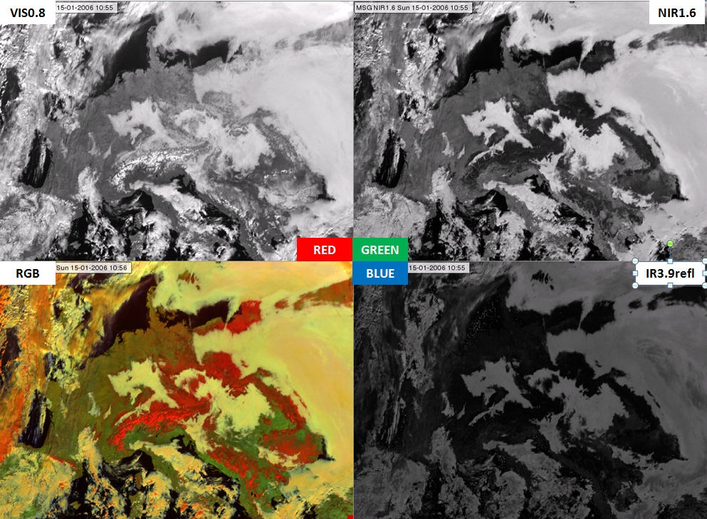
| Figure 3a: VIS0.8 (upper left), NIR1.6 (upper right), IR3.9refl (below right) images (all stretched within the 0-100 % reflectivity range) and the RGB created from these components (below left) for 15 January 2006 at 10:55 UTC |
|
Fig. 3a shows the VIS0.8, NIR1.6 and IR3.9refl images all visualized within the 0-100 % reflectivity ranges. The NIR1.6 image is darker than the VIS0.8 image and the IR3.9refl image is even darker. This is in accordance with Fig. 2 showing that the absorption of ice and water are much higher at 1.6 than at 0.8 micrometer and even higher at 3.9 micrometer. As a consequence the 0-100 % range seems to be NOT adequate for all three channels. For example, the blue channel seems to be too dark with this enhancement.
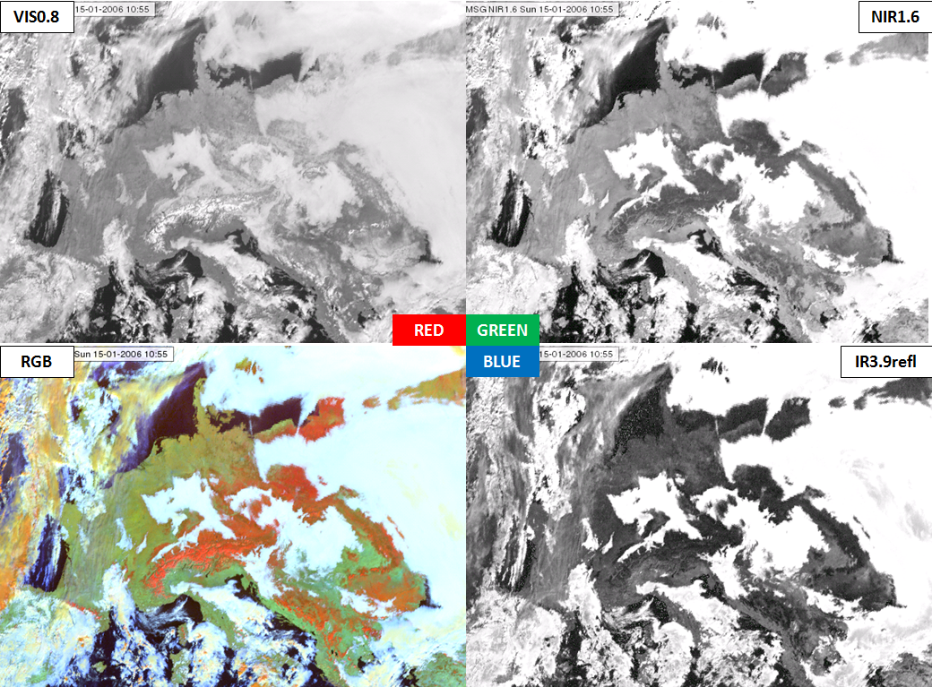
Fig. 3b shows the same images linearly stretched within the reflectivity ranges indicating in Table 1. The blue and the green colour components became brighter with the modified ranges. However, the snowy and snow-free land areas are not separated clearly enough in the IR3.9refl image.
| Figure 3b: VIS0.8 (upper left), NIR1.6 (upper right), IR3.9refl (below right) images, all stretched within the reflectivity ranges indicated in Table 1, and the RGB created from these components (below left) for 15 January 2006 at 10:55 UTC |

|
Fig. 3c shows the VIS0.8, NIR1.6 and IR3.9refl images enhanced according to the recipe of Table 1 (first linearly stretched and then gamma corrected). The snowy and snow-free land areas are separated clearly in the IR3.9refl image after the gamma correction.
| Figure 3c: VIS0.8 (upper left), NIR1.6 (upper right), IR3.9refl (bottom right) images, all stretched within the reflectivity ranges indicated in Table 1 and then gamma corrected, and the Snow RGB (bottom left) for 15 January 2006 at 10:55 UTC |
|
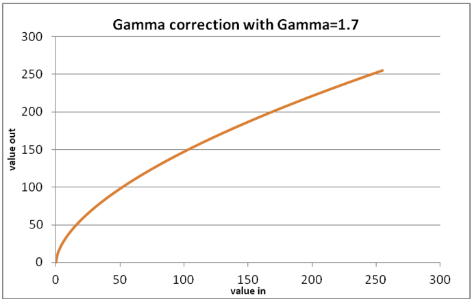
Why perform gamma correction? If a non-linear expansion is required, then gamma correction is performed after the linear stretching. The gamma correction enhances the contrast in the darker or in the brighter tones, depending on the Gamma parameter. In case of the Snow RGB (where Gamma is equal to 1.7), the contrast of the darker parts are increased, see Fig. 4.
| Figure 4: Effect of the gamma correction if the Gamma parameter is equal to 1.7 |
|
The bottom left panels of Figs. 3a, 3b and 3c show the RGB images created from the components presented on the corresponding figures. The bottom left panel of Fig. 3a shows the RGB when the components were linearly stretched in the 0-100 % reflectivity range. The bottom left panel of Fig. 3b shows the RGB when the components were linearly stretched in the ranges listed in Table 1. The bottom left panel of Fig. 3c shows the RGB when the components were first linearly stretched in ranges listed in Table 1, and then the gamma correction was applied. The last one is the Snow RGB. A comparison of these images shows how the RGB improves with proper enhancement.