Table of Contents
Cloud Structure In Satellite Images
As already mentioned in the general remarks, the cloud band of the occlusion described in this chapter develops in the area of a wave (see Wave ) However, the cloud band exhibits clearly different cloud layers, in contrast to the occlusion of the warm conveyor belt type (see Occlusion: Warm Conveyor Belt Type ).
In a fully developed stage, the satellite image shows two synoptic scale cloud bands:
- a multi-layered frontal cloud band associated with the cold front
- a lower cloud spiral which seems to penetrate from below the higher cloud band associated with the cold front
- both cloud bands seem to be uncoupled
Appearance in the basic channels:
- In the VIS image the cloud spiral is white indicating deep-layered cloudiness with high albedo.
- In the IR image the grey shades of a cold conveyor belt cloud band are more grey but with some
increased white areas overlaid. The following points can be summarized:
- At the boundary between the cloud band of the cold and warm front (oriented south-west to north-east) and the clouds associated with the cold conveyor belt type, a distinct gradient from white to (dark) grey can be observed. Often at some distance away from the boundary, cloud tops gradually become higher (whiter) followed again by a decrease of cloud-top heights within the innermost part of the cloud spiral. Such a cloud structure can be well explained with the conveyor belt theory (see Meteorological physical background ).
- During the later stages of development, high clouds can also develop leading to a similar appearance to the warm conveyor belt type of the occlusion (see Meteorological physical background ).
- In the WV image the two cloud bands with different cloud types are seen with even greater contrast. A black stripe characterising the dry air on the cyclonic side of the jet axis extends parallel to the higher cloud band and immediately crosses the cold conveyor belt cloudiness at the boundary. This effect cannot be detected in the case of an occlusion of the warm conveyor belt type. The driest air represented by darkest pixel values is included in the spiral development. This fact can be observed in both types of occlusion (see Occlusion: Warm Conveyor Belt Type ). During the later stages of development, high and therefore bright pixel values can be observed within the entire cloud spiral which means that the crossing black stripe is no longer visible.

Appearance in the basic RGBs:
Airmass RGB
The ccb occlusion cloud spiral and the connected cloud bands of the cold front and warm front form a synoptic scale frontal system. The ccb occlusion cloud spiral protrudes from below the WF cloudiness into the cold air trough and consequently exhibits lower cloud-tops heights.
The airmass RGB represents the warm and cold air masses in front of the frontal system with blue and green colours - depending on the geographical latitude. Green colours are more frequent in the southern areas. Behind the frontal cloud and the spiral cloud bands there are mostly brown colours, representing the sinking dry airmass. However, sometimes the colour here is blue, demonstrating that cold air exists.
In the airmass RGB, the cloud spiral of the ccb occlusion are very similar to the IR channels; often with a brownish shading exists above which demonstrates the overrunning dry air.
Dust RGB
The dust RGB appears in front of the frontal cloud band with mostly blue colours, representing the cloud free area; this can be blocked by other cloud areas. Behind the frontal cloud band and the ccb occlusion cloud spiral there are also some blue or pinkish blue areas where there is no cloud. However, there are typically also yellowish to ochre colours representing subsequent low cloudiness (cold air cloudiness and stratus).
In the Dust RGB the cold conveyor belt occlusion spiral shows a mixture of yellowish and red-brown areas; these colours are less intensive as those in the cloud band of the cold and warm front indicating lower cloud-top heights of the ccb occlusion spiral.
 |
 |
 |
|
Legend: Schematics for basic RGBs
Upper: Airmass RGB with full and partly dry air overrun; low: dust RGB
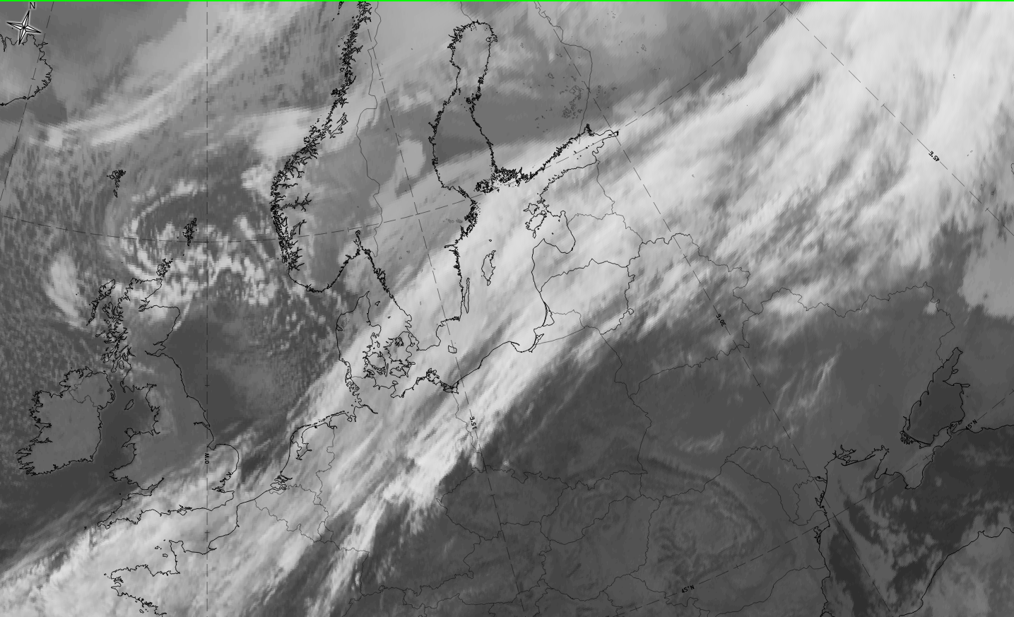
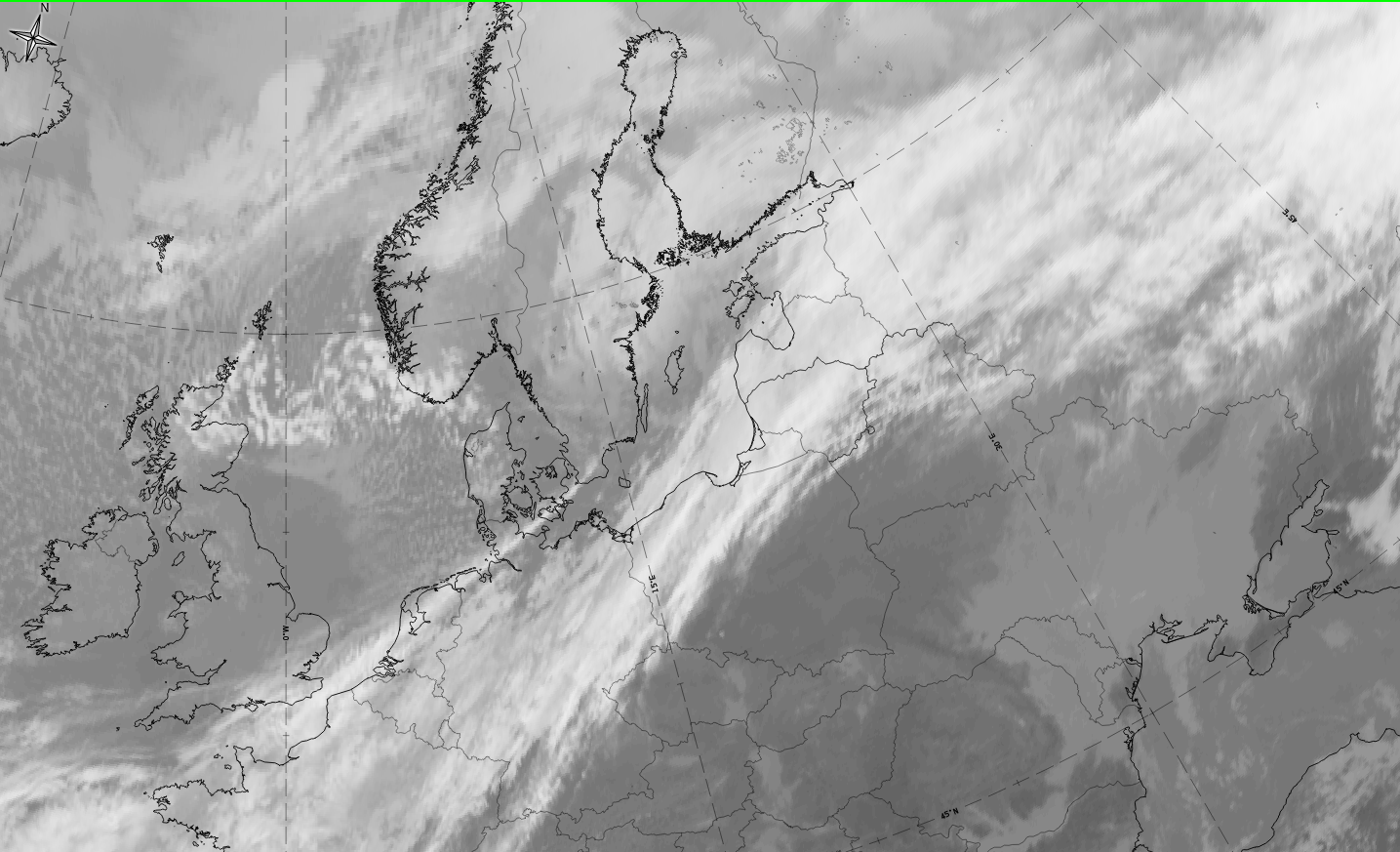
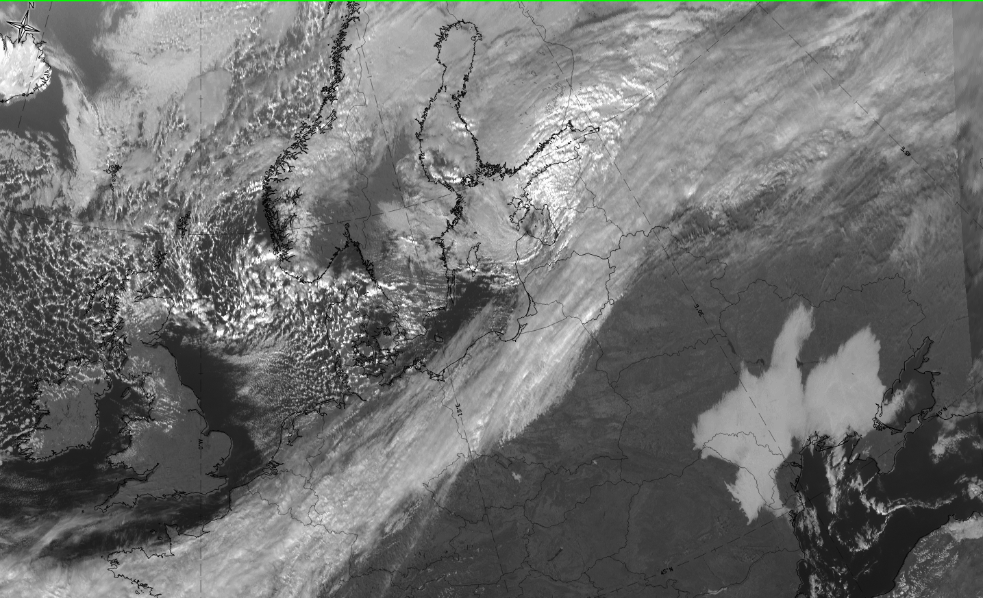
The case from 27 October 2019 shows the development from a wave at the CF - WF cloud system to a ccb spiral from South-Sweden, eastward to Finland and Russia. The IR image clearly shows the lower (greyer) cloud tops of the ccb spiral compared to the higher (whiter) cloud-top heights of the CF-WF band.
 |
 |
 |
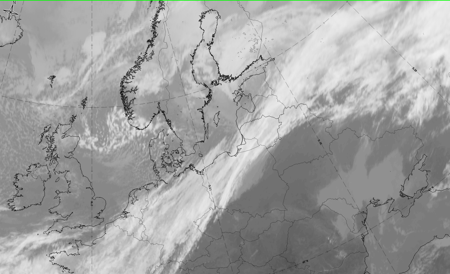 |
Legend: 27 October 2019; IR; u.l.:03 UTC; u.r.: 06 UTC; l.l.: 09UTC; l.r.: 12 UTC.
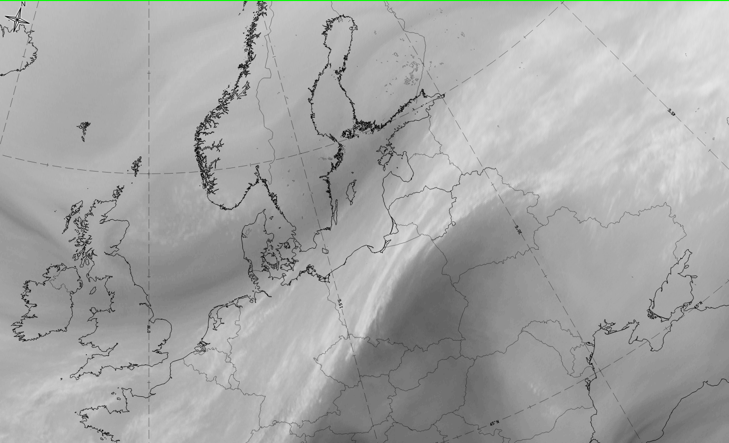
The fully developed stage of the ccb occlusion is presented here in all basic channels and also basic RGBs for 27 October 2019 at 12 UTC.
|
Hover over the image and move your pointer left and right to fade between images.Tap if using a touch interface. |
|
Hover over the image and move your pointer left and right to fade between images.Tap if using a touch interface. |
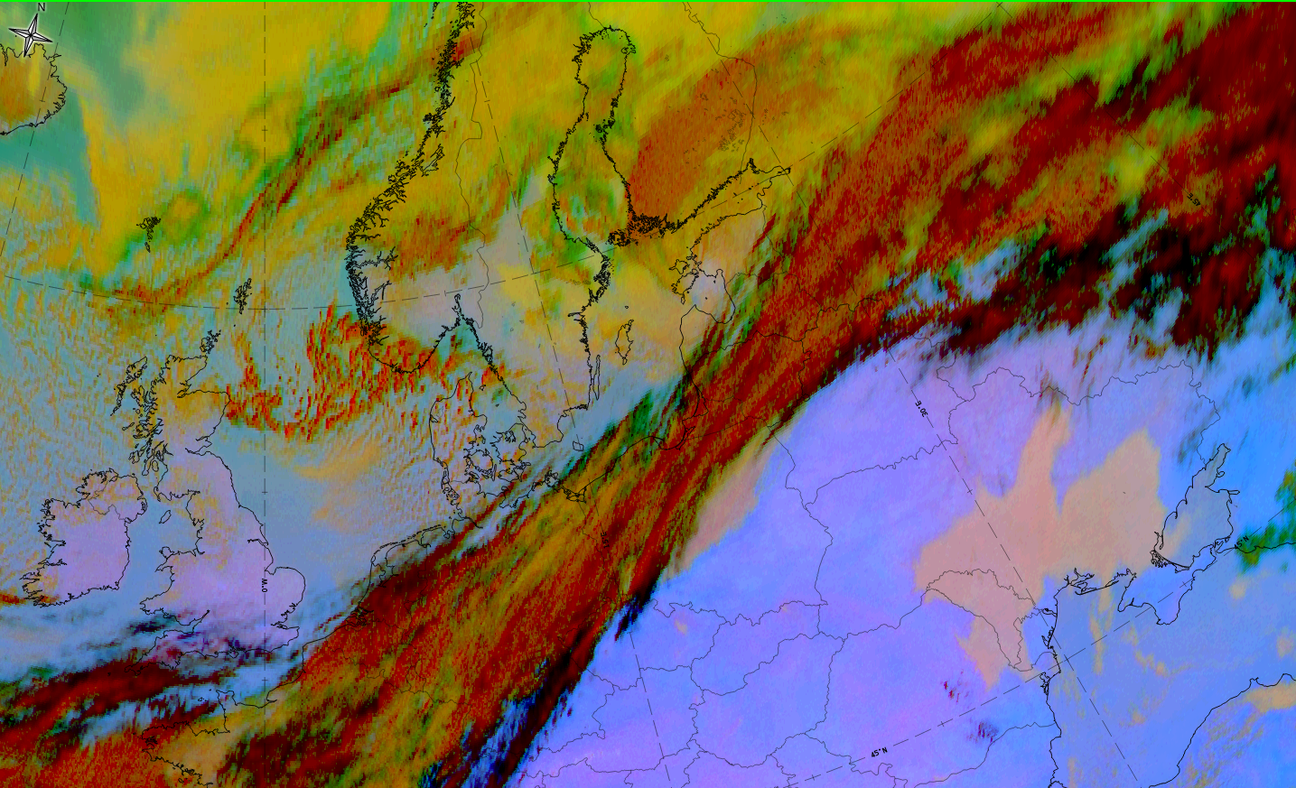
27 October2019, 12UTC: 1st row: IR (above) + HRV (below); 2nd row: WV (above) + Airmass RGB (below); 3rd row: Dust RGB + image gallery.
*Note: click on the Dust RGB image to access image gallery (navigate using arrows on keyboard)
| IR | Much greyer than the white CF-WF cloud band; brighter in the direction of the spiral tip to the Southwest. |
| HRV | Grey colours at this time of the year and at this high latitude; bright white colour in the inside of the spiral where solar illumination is better. |
| WV | Differentiation of grey shades between CF-WF band and ccb occlusion spiral is particularly distinct. |
| Airmass RGB | Dark brown stripe from the northeast, and along the rearward edge of the CF-WF band representing sinking, very dry air; it overflows the ccb occlusion spiral totally leading to red-brown colours there. |
| Dust RGB | Ochre colours of the ccb occlusion spiral clearly inside the CF-WF band and more and more dark-red colours further west and southwest of the cloud spiral. |
Meteorological Physical Background
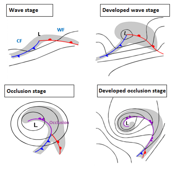
The classical Norwegian model
The classical development of an Occlusion (Warm Conveyor Belt Type) is described in the well-known polar Front theory after Bergeron as the development from a Wave to an Occlusion stage.
Deviations between cloud configurations in satellite images and the classical Norwegian model
There are Occlusion spirals which contradict the classical wave stage (shown above) as well as the overtaking mechanism completely. Those developments show a lower cloud spiral penetrating westward from below the Cold Front and Warm Front in the direction of the streaming (this is usually "westward" for a W-E moving system).
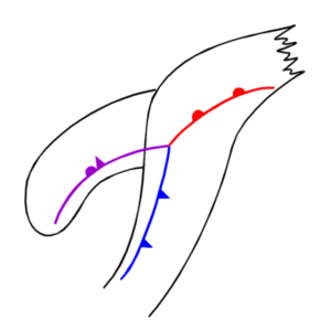
This type of occlusion cloud bands can much better be explained with the Conveyor Belt Model and - as the Cold Conveyor Belt manifests itself in form of a lower cloud spiral it is called a Cold Conveyor Occlusion in the Satellite Manual.
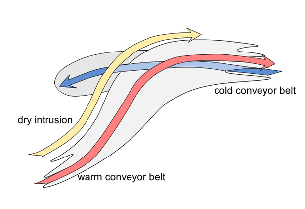
Conveyor Belt model
- The Cold Conveyor Belt
The lower levels of the troposphere are characterized by an ascending Cold Conveyor Belt, transporting moist and cool air ("cooler" compared with the Warm Conveyor Belt). As the Cold Conveyor Belt starts to rise in low layers from mostly east to west, it is below the Warm Conveyor Belt till it emerges at the western side and forms the lower cloud spiral of the Cold Conveyor Belt occlusion.
Further westward (in the direction of the stream) the tops of the Cold Conveyor Belt cloud spiral are becoming colder again as the Cold Conveyor Belt ascends there which changes for that part of the cloud spiral bending to the south: cloud tops become lower again as the Cold Conveyor Belt starts to descend there.
- The Warm Conveyor Belt
The mid- and upper levels of the troposphere are characterized by the moist and warm air within the Warm Conveyor Belt mainly at the anticyclonic side of the jet.
The Warm Conveyor Belt is parallel to the cloud band of the Cold Front and turns then anticyclonically parallel to the cloud band of the Warm Front (this is a difference from the Warm Conveyor Belt type of Occlusion (see Occlusion: Warm Conveyor Belt Type).
- The Dry Intrusion
The dry relative stream of the dry intrusion crosses the occlusion cloud spiral formed by the Cold Conveyor Belt at the cyclonic side of the jet in high levels. This situation restricts the development of higher cloudiness there and leads to the typical appearance in the satellite image (see Cloud structure in satellite image).
The vertical relation of these Conveyor Belts to each other
The dominant streams in this area are the Cold Conveyor Belt and the Warm Conveyor Belt.
|
|
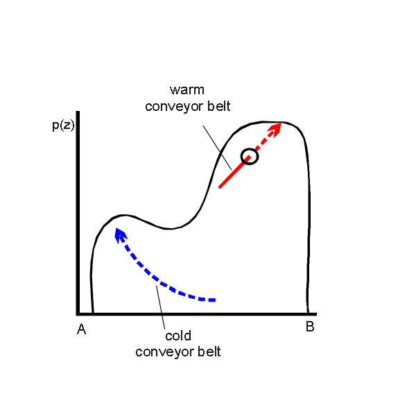
The lower cloud spiral develops in the rising Cold Conveyor Belt, while the higher cloud band of Warm Front and Cold Front are determined by the warm conveyor belt.
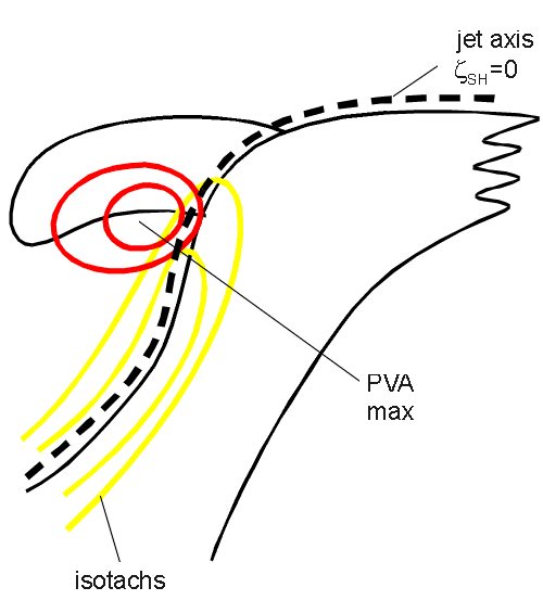
Relation between conveyor belts and Jet stream/streak
|
|
Such a distribution of conveyor belts can also be seen in relation to the upper level jet:
- The jet is parallel to the rear cloud edge of the cloud band of the Cold Front and further the leading edge of the Warm Front
- Often a jet streak exists with the CVA maximum within the left exit region; consequently this CVA maximum is superimposed on the cloud spiral of the Cold Conveyor Belt occlusion being responsible for thicker and more convective cloudiness there.
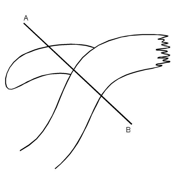
Below an example for the conveyor Belts on different (moist) isentropic surfaces for a Cold Conveyor Belt Occlusion can be seen.
|
21 June 2005/00.00 UTC - Meteosat 8 IR 10.8 image; position of vertical cross section A indicated
|
21 June 2005/00.00 UTC - Vertical cross section A; black: isentropes (ThetaE), blue: relative humidity, orange thin: IR pixel values, orange thick: WV pixel values
|

|
|
In cross section A, extending over the Atlantic from approximately 48N/34W to approximately 57N/34W, only the cold conveyor belt on the isentropic surface crosses the cross section perpendicularly. Humidity maxima and IR peaks contribute to the cold conveyor belt.
The relative streams cut the cross section perpendicularly on the isentropic surface of 314 K at a height between 650 and 850 hPa.
|
21 June 2005/00.00 UTC - Meteosat IR image; magenta: relative streams 314K - system velocity: 239° 18 m/s, yellow: isobars 328K; position of vertical cross section A indicated
|
21 June 2005/00.00 UTC - Meteosat 8 IR 10.8 image; position of vertical cross section B indicated
|

|

|
The cross section B is take perpendicular to the Warm Conveyor Belt. On the isentropic surface of 328K a rising warm conveyor belt can be observed. The relative streams of the Warm Conveyor Belt rise from 600 to 400 hPa and turn to the East and do not go into the direction of the occlusion.
|
21 June 2005/00.00 UTC - Vertical cross section; black: isentropes (ThetaE), blue: relative humidity, orange
thin: IR pixel values, orange thick: WV pixel values
|
21 June 2005/00.00 UTC - Meteosat IR image (ZAMG); magenta: relative streams 328K - system velocity: 239° 18 m/s, yellow: isobars 328K, position of vertical cross section B indicated
|
|
; magenta: relative streams 328K - system velocity: 239° 18 m/s, yellow: isobars 328K, position of vertical cross section B indicated")
|
The superimposed model fields of the isotachs and the PVA at 300 hPa are in quite good agreement with the ideal situation and can also be found in the former schematics.
|
21 June 2005/12.00 UTC - Meteosat 8 IR 10.8 image; yellow: isotachs 300 hPa, red: positive vorticity advection (PVA), black: zero line of shear vorticity 300 hPa
|
, black: zero line of shear vorticity 300 hPa")
|
Key Parameters
- Absolute topography at 500 and 1000 hPa:
The absolute topography at 1000 hPa is characterized by a low in the height field in the centre of the cloud spiral. At 500 hPa in the initial stages an upper level trough exists, which develops into an upper level low during a later stage of development. This is a main difference from the Warm Conveyor Belt Occlusion type where a closed cyclonic circulation already exists very early on (see Occlusion: Warm Conveyor Belt Type ). Consequently the Cold Conveyor Belt Type often changes to a Warm Conveyor Belt Type later on. - Equivalent thickness:
A prominent feature is the ridge of the equivalent thickness which is the consequence of the lifted warm air. In the case of well developed deep lows even a spiral structure of the ridge can be observed. But there are also situations which deviate from the distinct ridge structure. Well developed forms of Warm Front Occlusions and Cold Front Occlusions may lead to a more pronounced thickness gradient in the area of the Occlusion. This can be observed much better in the vertical cross section (see Typical appearance in vertical cross section). - Thermal front parameter (TFP):
The thermal front parameter mostly can be found close to the rear area of the cloud spiral. But the very existence of a front parameter depends on the existence of a pronounced temperature gradient. - Temperature advection:
The whole cloudiness of the Occlusion is under the influence of warm advection. The warm advection maximum can be found in the centre of the cloud spiral, mostly close to the point of the Occlusion. The zero line of the temperature advection follows the rearward edge of the Occlusion cloud spiral - Zero line of the shear vorticity at 300 hPa:
The zero line of the shear vorticity, which also indicates the jet axis, crosses the cloud spiral at the point of the Occlusion. - Isotachs at 300 hPa:
The jet axis crosses the frontal cloud band in the area of the point of the Occlusion as described above. If a well developed jet streak exists, the cold conveyor belt cloud spiral is situated within the area of the left exit region of this jet streak; consequently in the satellite image cellular structured colder cloud tops can be observed (see Cloud structure in satellite image). - Vorticity advection at 500 hPa and 300 hPa:
The cloud spiral of the occlusion is in general superimposed by PVA in the mid-levels and upper levels of the troposphere. As upper level troughs are involved, PVA is caused by both curvature and shear. But as described above the zero line of shear vorticity crosses the cloud spiral. The PVA maximum is very often situated within the left exit region of a jet streak (see Meteorological physical background and Weather events). There is a difference from the Warm Conveyor Belt Type of Occlusion, where curvature vorticity plays the dominant role (see Occlusion: Warm Conveyor Belt Type ).
In this case (21 June 2005) most of the numerical model fields fit quite well to the satellite image.
|
21 June 2005/12.00 UTC - Meteosat 8 IR 10.8 image; magenta: height contours 1000 hPa, cyan: height contours 500 hPa
|
|
|
|
|
21 June 2005/12.00 UTC - Meteosat 8 IR 10.8 image; blue: thermal front parameter 500/850 hPa, green: equivalent thickness 500/1000 hPa
|
|
|
|
|
21 June 2005/12.00 UTC - Meteosat 8 IR 10.8 image; blue: thermal front parameter 500/850 hPa, red: warm advection 500/1000 hPa
|
|

|
|
|
21 June 2005/12.00 UTC - Meteosat 8 IR 10.8 image; green: positive vorticity advection (PVA) 500 hPa
|
|
|
|
|
21 June 2005/12.00 UTC - Meteosat 8 IR 10.8 image; yellow: isotachs 300 hPa, black: zero line of shear vorticity 300 hPa, red: positive vorticity advection (PVA) 300 hPa
|
|

|

|
|
21 June 2005/12.00 UTC - Meteosat 8 IR 10.8 image; blue: shear vorticity 300 hPa, brown: curvature vorticity 300 hPa
|
|
|
|
Typical Appearance In Vertical Cross Sections
No notable difference could be found in the configuration of NWP parameters within vertical cross sections between Warm Conveyor Belt Occlusion and Cold Conveyor Belt Type.
The isentropes of the equivalent potential temperature generally show a distinct trough structure indicating the warmer air which has been lifted (see Meteorological physical background ) and the crowding zone of a surface front. In this case the upper level trough is forward inclined with height. The most frequent configuration is a Warm Front inclined crowding zone in front of the isentropic trough structure. The difference between the cross section of an Occlusion cloud band and of a Warm Front cloud band can be seen in the layer above the Warm Front surface: in a Warm Front case the isentropic trough configuration does not exist (see Warm Front Band , Warm Front Shield and Detached Warm Front ).

|
|
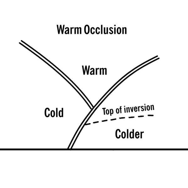
According to the sub-types Warm Occlusion Type, Cold Occlusion Type and Neutral Occlusion Type (see Occlusion: Warm Conveyor Belt Type - Key Parameters ) the following three vertical distributions of frontal zones can be expected.
|

|

|
In the investigation carried out by ZAMG two main different configurations could be observed:
- A Warm Front type: in this case the isentropic trough is forward inclined on top of the Warm Front zone.
- A Warm Front inclined crowding zone in front of and a Cold Front inclined crowding zone behind, the isentropic trough feature. In this case the forward inclination of the isentropic trough is not as strongly pronounced as in the other case. Sometimes also a straight vertical trough axis can be observed.
|
|
The field of the relative humidity is characterized by high values, of about 80% and even more, within the area of the isentropic trough. In the case of a forward inclined trough the maximum values of the humidity have forward inclination, two low values of relative humidity can be observed within and below the lower isentropes of the Warm Front - like crowding zone. This minimum typically is situated between approximately 800 and 700 hPa. A second minimum of the relative humidity can be found on the rear side of the isentropic trough within the upper levels of the troposphere at approximately 300 hPa. This corresponds to the following dry intrusion.
The whole area of the Warm Front inclined crowding zone and the leading part of the isentropic trough feature is under the influence of pronounced WA. The maximum of WA mostly can be found within the lower levels of the troposphere very close to the area where the Warm Front inclined crowding zone reaches the surface. A secondary pronounced area of WA can be found within the upper levels of the troposphere on the rear side of the isentropic trough. This area is typically situated at approximately 300 hPa and indicates the tropopause. The lower and mid-levels of the troposphere are characterized by pronounced CA. The zero line of temperature advection is close to the minimum of the isentropic trough in the lower and mid-levels of the troposphere. Very often the zero line in these levels is characterized by a forward inclination which leads to the development of a potentially unstable stratification of the troposphere (see Meteorological physical background and Key parameter).
The field of vorticity advection is characterized by PVA within the whole area of the Occlusion. Typically two PVA maxima can be found in the cross section. The main maximum exists in the upper levels of the troposphere on the rear side of the isentropic trough and is connected with the left exit region of a jet streak; a weaker PVA maximum exists within the Warm Front inclined crowding zone in the lower levels of the troposphere at approximately 800 hPa. This maximum is connected with the already pronounced cyclonic circulation in these levels and indicates the propagation of the low area (see Meteorological physical background and Key parameters).
The field of divergence shows pronounced convergence within the area of the Warm Front inclined crowding zone and within the lower part of the leading area of the isentropic trough configuration. In the upper part divergence prevails. The zero line of divergence can be found very close to the trough axis.
According to the distribution of convergence, temperature advection and vorticity advection, the field of vertical motion (omega) shows a wide area of strong upward motion within the area of the occlusion. The strongest upward motion typically can be found within the mid-levels of the troposphere.
In the VIS image the whole frontal cloud band is characterized by high pixel values. In contrast to this the pixel values in the IR and WV images depend on the location of the cross section as well as on the stage of development. During the initial stages the pixel values of the IR and WV images within the area of the dry intrusion, close to the point of the Occlusion, are characterized by lower values typical for low and mid-level cloudiness. Downstream of the cloud spiral the pixel values are increasing continuously. During the maturing stages, when the cloud spiral is also accompanied by high cloudiness within the whole cloud spiral, the pixel values are as high as in case of an Occlusion of the Warm Conveyor Belt type (see Occlusion: Warm Conveyor Belt Type ).
|
21 June 2005/00.00 UTC - Meteosat 8 IR 10.8 image; position of vertical cross section indicated
|
|

|

|
|
21 June 2005/00.00 UTC - Vertical cross section; black: isentropes (ThetaE), blue: relative humidity, orange thin: IR pixel values, orange thick: WV pixel values
|
|
|

|
|
21 June 2005/00.00 UTC - Vertical cross section; black: isentropes (ThetaE), red thick: temperature advection - WA, red thin: temperature advection - CA, orange thin: IR pixel values, orange thick: WV pixel values
|
|

|

|
|
21 June 2005/00.00 UTC - Vertical cross section; black: isentropes (ThetaE), green thick: vorticity advection - PVA, green thin: vorticity advection - NVA, orange thin: IR pixel values, orange thick: WV pixel values
|
|
|

|
|
21 June 2005/00.00 UTC - Vertical cross section; black: isentropes (ThetaE), magenta thin: divergence, magenta thick: convergence, orange thin: IR pixel values, orange thick: WV pixel values
|
|

|
|
|
21 June 2005/00.00 UTC - Vertical cross section; black: isentropes (ThetaE), cyan thick: vertical motion (omega) - upward motion, cyan thin: vertical motion (omega) - downward motion, orange thin: IR pixel values, orange thick: WV pixel values
|
|
|
|
The isentropes show an inclined crowding zone similar to a Warm Front with unstable behaviour within the lower levels of the troposphere and an isentropic trough configuration which is forward inclined. High values of humidity can be found forward inclined within the leading part of the trough, humidity minima within the Warm Front inclined crowding zone at approximately 500 hPa and at the rear side of the Occlusion cloud band at approximately 300 hPa. The latter represents the dry intrusion. The field of temperature advection shows strong WA within the leading part of the Occlusion and strong CA within the rear part of the Occlusion. The zero line within the lower and mid-levels of the troposphere has a forward inclination which leads to the development of a potentially unstable stratification of the troposphere. The field of vorticity advection contains only the high level PVA maximum mentioned above: a PVA maximum at approximately 400 hPa at the rearward edge of the cloud band (around 34W48N). However within the lower levels, between approximately 600 and 800 hPa, there is some PVA, but a typical PVA maximum is not seen. The main feature in the field of divergence is a pronounced convergence zone within the lower layers of the Occlusion trough extending upward in the Warm Front - like crowding zone. Pronounced divergence can be found above this zone. The field of omega shows strong upward motion within the whole area of the Occlusion.
Weather Events
| Parameter | Description |
| Precipitation |
|
| Temperature |
|
| Wind (incl. gusts) |
|
| Other relevant information |
|
|
Hover over the image and move your pointer left and right to fade between images.Tap if using a touch interface. |
27 October 2019, 12UTC: IR + synoptic measurements (above) + probability of moderate rain (Precipitting clouds PC - NWCSAF)
Note: for a larger SYNOP image click this link.
The synoptic measurements correspond very well to the schematic representing the ideal situation. Many stations report precipitation, but the higher intensity can be found more in the CF-WF area than in the occlusion spiral. Showery precipitation and Cb reports are associated with the ccb spiral closest to the CF-WF boundary and less intensive rain is associated with the southwestern part of the occlusion spiral. This corresponds to the values of PC (probability of moderate precipitation) which are low but have higher values in this area
|
Hover over the image and move your pointer left and right to fade between images.Tap if using a touch interface. |
|
Hover over the image and move your pointer left and right to fade between images.Tap if using a touch interface. |
27 October 2019, 12 UTC
1st row: Cloud Type (CT NWCSAF) (above) + Cloud Top Height (CTTH - NWCSAF) (below); 2nd row: Convective Rainfall Rate (CRR NWCSAF) (above) + Radar intensities from Opera radar system (below).
For identifying values for Cloud type (CT), Cloud type height (CTTH), precipitating clouds (PC), and Opera radar for any pixel in the images look into the legends. (link).
References
General Meteorology and Basics
- BENNETTS D. A., GRANT J. R. and MCCALLUM E. (1988): An introductory review of fronts. Part I: Theory and observations; Met. Mag., Vol. 117, p. 357 - 370
- BENNETTS D. A., GRANT J. R. and MCCALLUM E. (1989): An introductory review of fronts. Part II: A case study; Met. Mag., Vol. 118, p. 8 - 12
- CONWAY B. J., GERARD L., LABROUSSE J., LILJAS E., SENESI S., SUNDE J. and ZWATZ-MEISE V. (1996): COST78 Meteorology - Nowcasting, a survey of current knowledge, techniques and practice; Phase 1 report; Office for official publications of the European Communities
General Satellite Meteorology
- BADER M. J., FORBES G. S., GRANT J. R., LILLEY R. B. E. and WATERS A. J. (1995): Images in weather forecasting - A practical guide for interpreting satellite and radar imagery; Cambridge University Press
- CARLSON T. N. (1987): Cloud configuration in relation to relative isentropic motion; in: Satellite and radar imagery interpretation, preprints for a workshop on satellite and radar imagery interpretation - Meteorological Office College, Shinfield Park, Reading, Berkshire, England, 20 - 24 July 1987, p. 43 - 61
- EVANS M. S., KEYSER D., BOSART L. F. and LACKMANN G. M. (1994): A satellite derived classification scheme for rapid maritime cyclogenesis; Mon. Wea. Rev., Vol. 122, p. 1381 - 1416
Specific Satellite Meteorology
- BROWNING K. A. (1985): Conceptual models of precipitation systems; Met. Mag., Vol. 114, p. 293 - 317
- BROWNING K. A. and HILL F. F. (1985): Mesoscale analysis of a polar trough interacting with a polar front; Quart. J. R. Meteor. Soc., Vol. 111, p. 445 - 462
- BROWNING K. A. (1986): Conceptual models of precipitation systems; Weather&Forecasting, Vol. 1, p. 23 - 41
- BROWNING K. A. (1990): Organization of clouds and precipitation in extratropical cyclones; in: Extratropical Cyclones, The Erik Palmen Memorial Volume, Ed. Chester Newton and Eero O Holopainen, p. 129 - 153
- CARLSON T. N. (1980): Airflow trough mid-latitude cyclones and the comma cloud pattern; Mon. Wea. Rev., Vol. 108, p. 1498 - 1509
- GREEN J. S. A., LUDLAM F. H. and MCILVEEN J. F. R. (1966): Isentropic relative - flow analysis and the parcel theory; Quart. J. R. Meteor. Soc., Vol. 92, p. 210 - 219
- REED R. J. (1990): Advances in knowledge and understanding of extratropical cyclones during the past quarter century: an overview; in: Extratropical Cyclones, The Erik Palmen Memorial Volume, Ed. Chester Newton and Eero O Holopainen, p. 27 - 45
- THEPENIER R.-M. and CRUETTE D. (1981): Formation of cloud bands associated with the American subtropical jet stream and their interaction with mid-latitude synoptic disturbances reaching Europe; Mon. Wea. Rev., Vol. 109, p. 2209 - 2220
Special Investigation: T-Bone
A T-bone is a frontal structure seen during a special development of a deepening low. It was first identified in 1990 by Shapiro and Keyser. The main feature of the cloudiness in a T-bone is that the Cold and Warm Fronts are separated from each other; the Cold Front near the low centre weakens, whereas the Warm Front and the Cold Front farther away strengthen. T-bones develop usually over the sea in wintertime in a strong zonal flow with a flat and confluent upper level trough. The name "T-bone" comes from the frontal fracture stage, where the Cold Front and the Warm Front are separated and perpendicular to each other.
From satellite image and conceptual model points of view, the T-bone is a special case of a Cold Conveyor Belt Occlusion. Both start as a Wave in a baroclinic zone and end as an Occlusion. There are, however, significant differences in the stages in between. T-bones can also be seen as a type of Rapid Cyclogenesis (see Rapid Cyclogenesis ), because a deep surface low with strong winds and a typical cloud head development are observed. There is also a dissipation of cloudiness in the gap between the fronts due to the effect of a right exit region of a jet, which is similar to the conceptual model Front Decay (see Front Decay ). Also, because the Cold Front is weak at lower levels, T-bone has features similar to an upper Cold Front (see Cold Front ).
In this chapter two cases are compared: a Cold Conveyor Belt Occlusion 05 - 06 January 2003 and a T-bone 01 - 02 April 2001; the main differences are presented.
The T-bone development stages are presented in the following schematics:
|
As there are no significant differences in the Wave and occluded stages, only the changes that occur during the cloud head and cloud hook stages are discussed here.
Satellite Images
Appearance of a Cold Conveyor Belt Occlusion in satellite images:
In IR images a lower cloud spiral gradually appears from below the higher cloud band. There is a dark area between Cold and Warm frontal cloudiness and the cloud head.
In WV images a Dark Stripe behind the Cold Front crosses the cold conveyor belt near the Occlusion point.
|
|

|

|
|
05 January 2003/18.00 UTC - Meteosat IR image
|
05 January 2003/18.00 UTC - Meteosat WV image
|
Appearance of a T-Bone in satellite images:
In tha IR images below, a weak lower cloud spiral seems to exist before the Occlusion. In the cloud head and cloud hook stages the cold frontal clouds clearly dissolve near the Warm Front due to the frontal fracture and the effect of the right exit area of the jet stream.
In the WV images below, there is a Dark Stripe behind the Cold Front, but it does not cross it as in the case of the Cold Conveyor Belt Occlusion. The Cold Front near the surface low is very dark grey in WV images.
|
|

|

|
|
01 April 2001/18.00 UTC - Meteosat IR image
|
01 April 2001/18.00 UTC - Meteosat WV image
|
The Cold Conveyor Belt Occlusion case:
The loop shows IR images from 05 January 12.00 UTC to 06 January 00.00 UTC. In the upper left corner there is a Wave that moves eastwards and develops into a Cold Conveyor Belt Occlusion, although there are also some features of Rapid Cyclogenesis present. The cloud head stage is reached on 05 January 18.00 UTC and the cloud hook stage on 06 January 00.00 UTC. The depression occludes on 06 January 00.00 UTC.
|
05 January 2003/12.00 UTC - Meteosat IR image
|
|
 Loop: 05/18.00 - 06/00.00 UTC hourly image loop Loop: 05/18.00 - 06/00.00 UTC hourly image loop
|
The T-bone case:
The loop below shows IR images from 01 April 15.00 UTC to 02 April 10.00 UTC. There is a Wave over the Atlantic that moves towars the British Isles and develops into a Warm Occlusion (for the of Occlusions see Meteorological Physical Background). The cloud head stage is reached at 18.00 UTC on 01 April and the cloud hook stage between 00.00 - 06.00 UTC on 02 April. By 02 April 12.00 UTC the depression has occluded.
|
01 April 2003/15.00 UTC - Meteosat IR image
|

|
|
Loop: 01/15.00 - 02/10.00 UTC hourly image loop
|
Numerical Parameters
The height contours of 1000 and 500 hPa are similar in both cases: i.e. a rapidly deepening surface low with an upper trough to the west.
Temperature advection is, likewise, similar: the Warm Front and the cloud head cloud systems are within warm advection in both cases.
Jet stream:
In the case of the Cold Conveyor Belt Occlusion there is a strong jet following the cyclonic edge of the frontal cloudiness. In the T-Bone, there are two jets: one ahead of the Warm Front and a second behind the Cold Front. In the frontal fracture stage they are separated, in the Occlusion stage the two jets merge.
Zero line of shear vorticity at 300 hPa:
In the Cold Conveyor Belt Occlusion the zero line of shear vorticity is a relatively straight line following the jet streak. In the T-Bone the zero line is curveed within the cloud head and cloud hook. The curve straightens somewhat in the Occlusion stage.
|
05 January 2003/18.00 UTC - Meteosat IR image; yellow: isotachs 300 hPa, black: zero line of shear vorticity 300 hPa
|
01 April 2001/18.00 UTC - Meteosat IR image; yellow: isotachs 300 hPa, black: zero line of shear vorticity 300 hPa
|
|
|
Vertical Cross Sections
The cross sections below are taken during the cloud head stage. They show the properties of the partly dissolved Cold Front, which is the main difference between Cold Conveyor Belt Occlusion and a T-bone.
The cross section is taken through the partly dissolved Cold Front near the surface low. The Cold Front is seen on the left, approximately in the area between longitudes 18W and 12W. The cross sections show:
- Weak Cold Front structure in the isentropes below 600 hPa between longitudes 18W and 16W with low IR and WV signals, and a weak upper Cold Front between 16W and 12W with higher IR and WV signals
- Warm advection in the area of Cold Front in the lower troposphere, very weak cold advection in the area of the upper Cold Front
- Very strong rising motion in the area of the front, not ahead and behind it as in a Cold Front (see Cold Front - Typical appearance in vertical cross sections )
- High humidity throughout the frontal zone
It can be concluded that although there is a weak cold frontal structure, the parameters do not fit a Cold Front.
|
01 April 2001/18.00 UTC - Meteosat IR image; position of vertical cross section indicated
|
01 April 2001/18.00 UTC - Vertical cross section; black: isentropes (ThetaE), red thick: temperature advection - WA, red thin: temperature advection - CA, orange thin: IR pixel values, orange thick: WV pixel values
|
|
|
|
|
|
01 April 2001/18.00 UTC - Vertical cross section; black: isentropes (ThetaE), cyan thick: vertical motion (omega) - upward motion, cyan thin: vertical motion (omega) - downward motion, orange thin: IR pixel values, orange thick: WV pixel values
|
01 April 2001/18.00 UTC - Vertical cross section; black: isentropes (ThetaE), blue: relative humidity, orange thin: IR pixel values, orange thick: WV pixel values
|
Weather Events
T-Bones are frontal structures that are usually associated with rapidly deepening lows. Heavy rain occurs ahead of the Warm Front, and stormy winds around its tail, especially in systems over the ocean. Contrary to a Cold Conveyor Belt Occlusion, there is no precipitation associated with the Cold Front located near to the Warm Front.

|
|