Table of Contents
Cloud Structure In Satellite Images
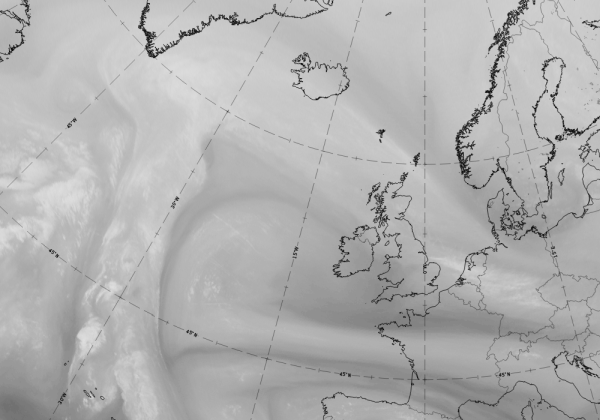
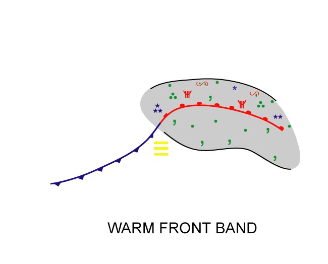
The satellite image shows an anticyclonically curved synoptic-scale cloud band, connected to a cold front cloud band.
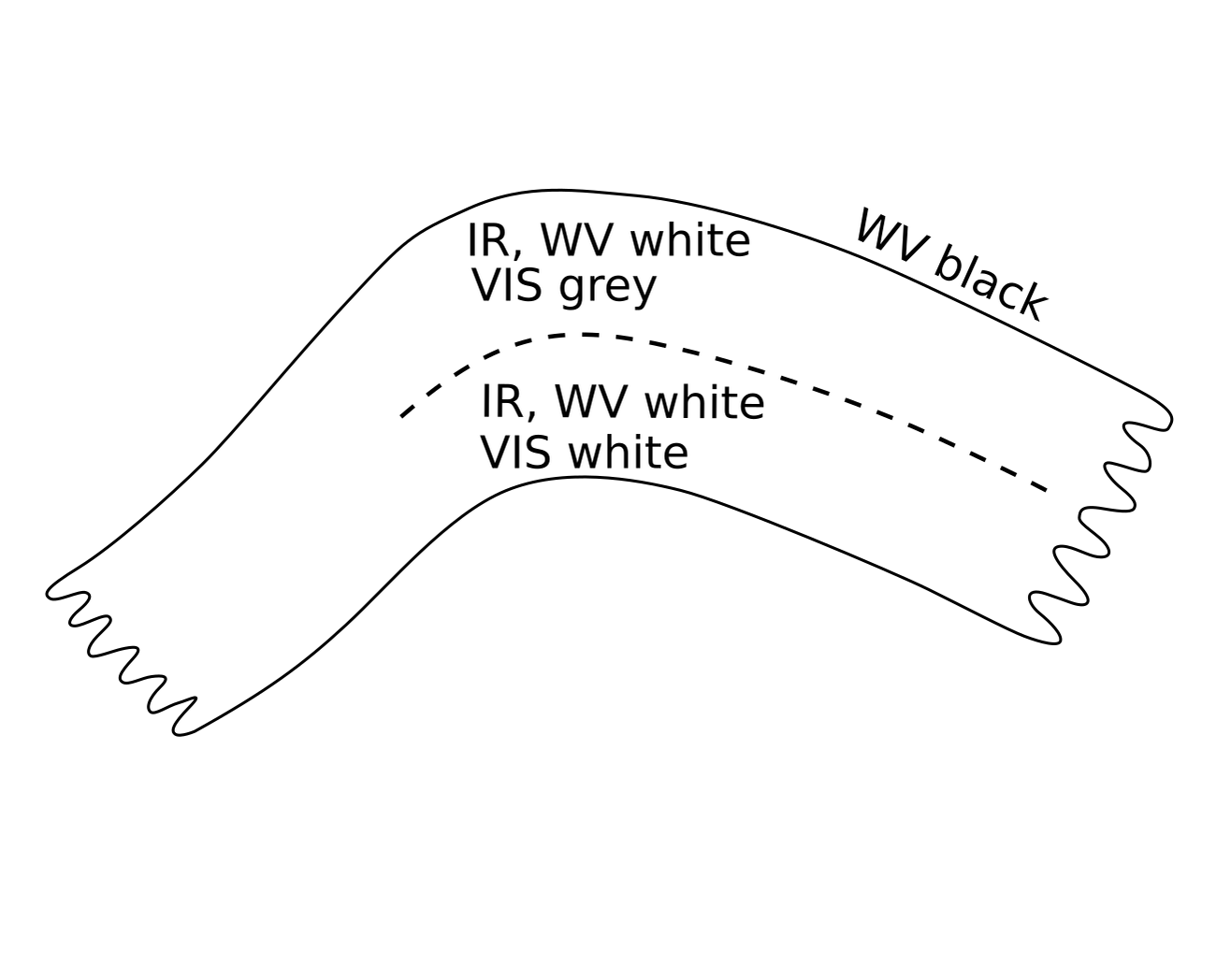
Appearance in the basic channels
- In ideal cases:
- in the VIS image the grey shades are generally bright at the rear edge becoming increasingly grey and dimmer towards the forward edge;
- in the IR image the grey shades of the cloud band are grey-white; in the ideal case, the brighter pixel values exist towards the forward and downstream cloud edge.
- In reality:
- very often no continuous cloud band exists but rather there are several cloud layers with broken clouds. Sometimes only high clouds exist;
- in the IR image several high-level white cloud areas overlay the lower, grey cloud layers (see Meteorological Physical Background).
- High and bright WV pixel values can be observed in the area of the frontal cloud band region.
- At the leading edge of the cloud band the WV image shows a sharp gradient from white to black indicating dry air along the cyclonic side of the jet.
Appearance in the basic RGBs:
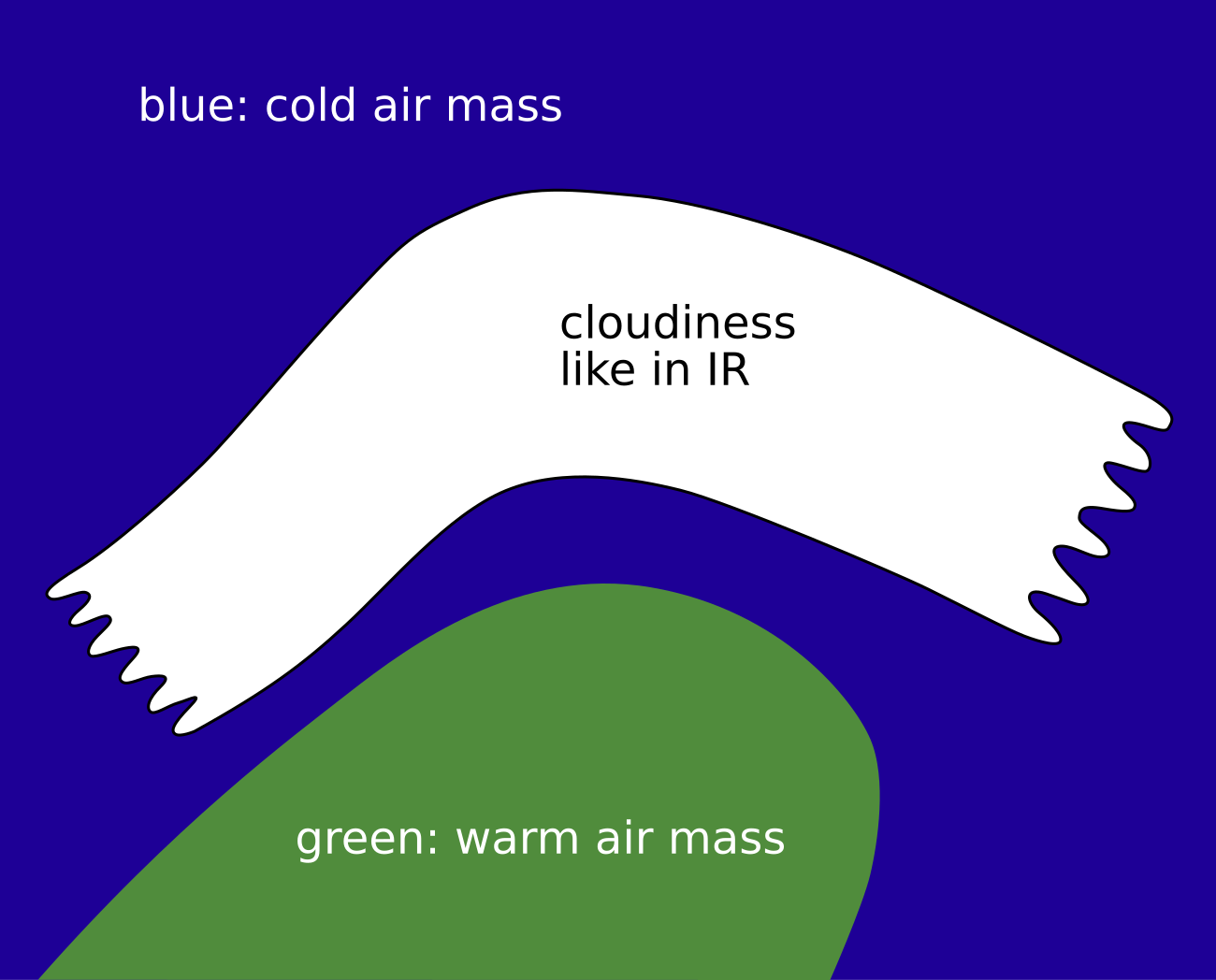
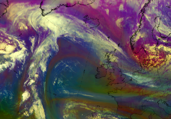
Airmass RGB
In front of the WF band blue colours indicate cold air masses and are a common feature. At the rear side, within the warm sector, the colour varies with a gentle gradient from greenish colours (representing warm air masses) to blue colours close to the rear edge of the WF band. The blue colours represent the frontal upgliding of warmer air over the originally cold air mass, as well as high humidity in upper-levels in these regions.
The texture of the clouds in the warm front band is very similar to their appearance in the IR image.
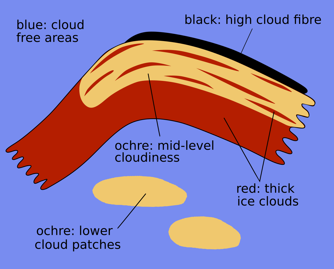
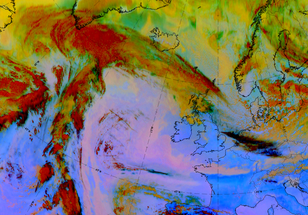
Dust RGB
Blue to pinkish-blue colours can be seen where there is cloud free land or sea exists. There are other cloud patches, which exist in front of the cloud band and also in the warm sector. These are usually lower, especially in winter time when fog and stratus fields occur. These cloud configurations appear in different shades of ochre.
In the warm front band, the colours are dependent upon the thickness of the cloud. Thicker areas appear dark red (indicating thick ice cloud), lower cloud appear in yellow to ochre. Quite often the leading edge of the warm front cloud band is accompanied by a black filament or fibres which accompany the jet axis region.
 |
 |
Legend: schematics for basic RGBs; Left: airmass RGB; right: dust RGB.
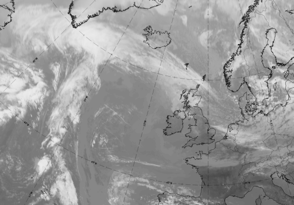
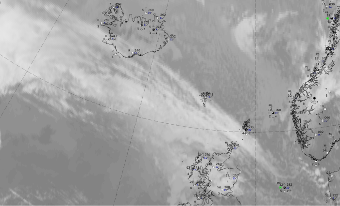
The case from 17 September 2019 at 12 UTC demonstrates a good example of a WF cloud band extending from the Atlantic, just south of Greenland and Iceland over to Northern Scotland.
|
|

|
|
Legend: 17 September 2019 at 12UTC: 1st row: IR (above) + HRV (below); 2nd row: WV (above) + Airmass RGB (below); 3rd row: Dust RGB + image gallery.
*Note: click on the Dust RGB image to access image gallery (navigate using arrows on keyboard).
| IR | Bright colours; a bright cloud filament or fibres at the leading edge. |
| HRV | Bright colours at the rearward edge of the cloud band. |
| WV | Bright band of high humidity with the bright cloud fibre at the leading edge; a dark stripe in advance of the cloud fibre. |
| Airmass RGB | Blue colours within and around the cloud band which indicate cold air; cloud patterns and textures similar to IR. |
| Dust RGB | Ochre colours indicate mid-level clouds; red stripes overlay thicker ice clouds; the stripe at the leading edge appears darker, almost black, indicating thin translucent high cloud. |
Meteorological Physical Background
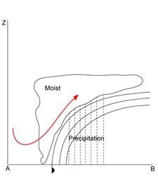
In the case of a Warm Front, warm moist air moves against colder dry air. At the boundary of these two air masses the warm air tends to slide up over the wedge of colder air (see Typical Appearance In Vertical Cross Sections). This process causes the frontal cloud band, and the associated precipitation, found mainly in front of the surface front (or the TFP) (see Weather events).
|
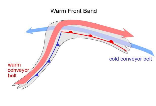
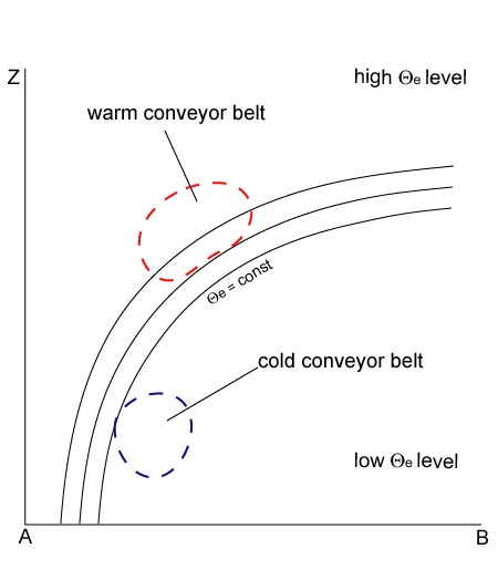
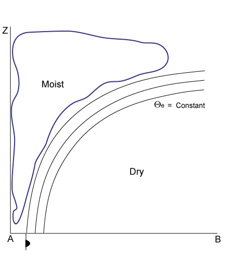
The idealized structure and physical background of a Warm Front can be explained with the conveyor belt theory as follows:
- Frontal cloud band and precipitation are in general determined by the ascending Warm Conveyor Belt, which has its greatest upward motion between 700 and 500 hPa. The Warm Conveyor Belt starts behind the frontal surface in the lower levels of the troposphere, crosses the surface front and rises to the upper levels of the troposphere. There the Warm Conveyor Belt turns to the right (anticyclonically) and stops rising, when the relative wind turns to a direction parallel to the front. If there is enough humidity in the atmosphere, the result of this ascending Warm Conveyor Belt is condensation and more and more higher cloudiness.
- The Cold Conveyor Belt in the lower layers, approaching the Warm Front perpendicularly in a descending motion, turns immediately in front of the surface Warm Front parallel to the surface front line. From there on the Cold Conveyor Belt ascends parallel to the Warm Front below the Warm Conveyor Belt. Due to the evaporation of the precipitation from the Warm Conveyor Belt within the less moist air of the Cold Conveyor Belt, the latter quickly becomes moister and saturation may occur with the consequence of a possible merging of the cloud systems of Warm and Cold Conveyor Belt to form a dense nimbostratus.
Discussion
In addition to this idealized structure, the experience from a series of case studies carried out at ZAMG differs somewhat from the one described above, allowing more differentiation. In the case of a band type the Warm Conveyor Belt can be observed within the warm sector up to the Cold and Warm Front line. If there is high cloudiness in front of and parallel to the Warm Front line, it is situated within an (at least in the area of the fronts) ascending conveyor belt from the rear side of the Cold Front extending from south-west to north-east, the so-called upper relative stream. While the high cloudiness can thus be explained, the Warm Front cloudiness in the lower levels of the troposphere develops, as in the ideal case described above, within the Cold Conveyor Belt.
The conveyor belt situation, especially of the Warm Conveyor Belt and the upper relative stream, described above can be found in a thick layer of isentropic surfaces, but there is some tendency for the Warm Conveyor Belt in lower layers to overrun the surface Warm Front to a small extent. The ascending Warm Conveyor Belt in the warm sector is not accompanied by appreciable cloudiness either because of too dry air masses or/and too little lifting. But it can be observed that in the ascending Warm Conveyor Belt cloudiness may develop leading to a second Warm Front type, the Warm Front Shield.
|
|
Very often a transition from the Warm Front Band to the Warm Front Shield can be observed by the development of cloudiness within the warm sector. This is described in detail in the chapter of the Warm Front Shield (see Warm Front Shield - Meteorological physical background ).
|
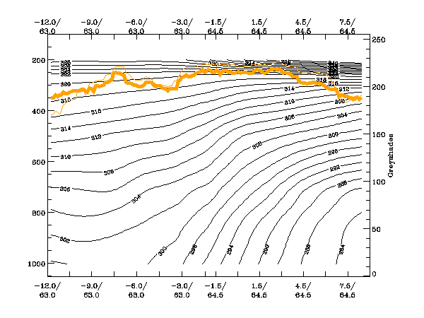
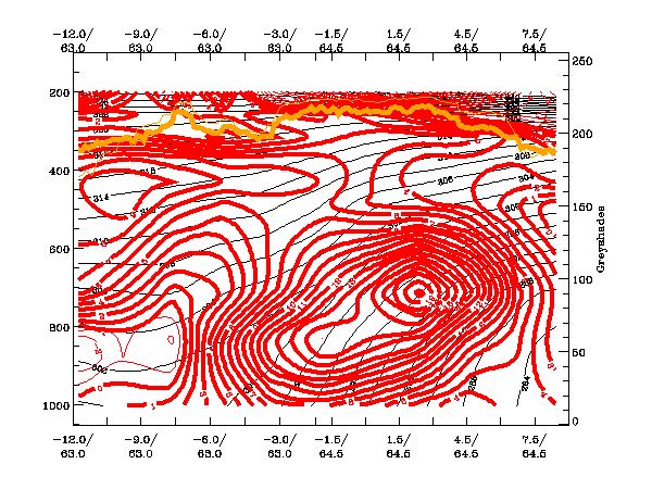
14 November 2004/00.00 UTC - Vertical cross section; black: isentropes (ThetaE), orange thin: IR pixel values, orange thick: WV pixel values
|
|
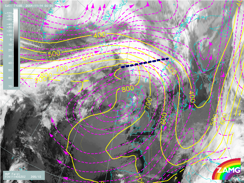
The 302K isentropic surface chosen for the relative streams in the figure below is very close to the upper boundary of the higher gradient, inclined Warm Front zone.
|
14 November 2004/00.00 UTC - Meteosat 8 IR 10.8 image; magenta: relative streams 302K - system velocity: 295° 10 m/s, yellow: isobars 300K, position of vertical cross section indicated
|
|
The analysis shows two Conveyor Belts: there is one from eastern directions across The Netherlands, Belgium, France, turning northward in an anticyclonic direction over the Atlantic. This is a typical example of a Warm Conveyor Belt extending across the warm sector to the leading edge of the Cold Front and the rear edge of the Warm Front cloudiness. A second relative stream originates from the cold air mass over the Atlantic behind the Cold Front and approaches the Warm Conveyor Belt over Iceland, extending from there on across the Atlantic (approx. 66N/2W) towards Norway parallel to the Warm Conveyor Belt. Generally speaking, the Warm Conveyor Belt rises from about 800 hPa over the Atlantic up to 400 hPa over Norway. The relative stream from the Atlantic exists in a higher layer, rising from about 600 to 450 hPa. The high cloudiness of the Warm Front exists in this latter relative stream.
|
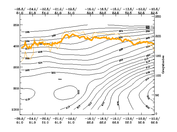
15 September 2004/06.00 UTC - Vertical cross section; black: isentropes (ThetaE), orange thin: IR pixel values, orange thick: WV pixel values
|
|
The isentropic surfaces which are used for the relative streams are 318K, which represents the situation within the lower levels of the troposphere, and 326K which is characteristic for the upper levels.
|
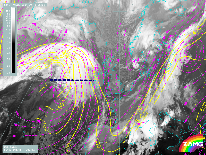
15 September 2004/06.00 UTC - Meteosat 8 IR 10.8 image; magenta: relative streams 318K - system velocity: 252°
13 m/s, yellow: isobars 318K, position of vertical cross section indicated
|
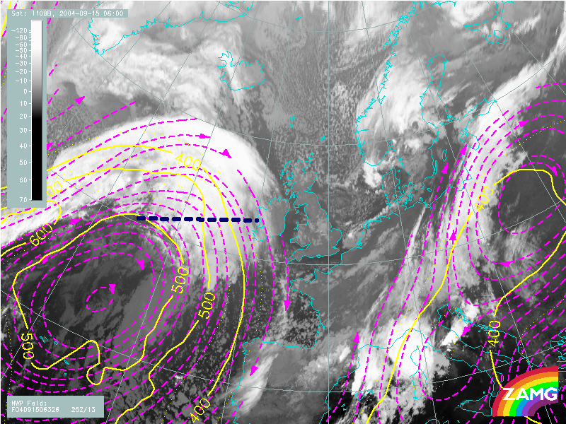
15 September 2004/06.00 UTC - Meteosat 8 IR 10.8 image; magenta: relative streams 326K - system velocity: 252? 13 m/s, yellow: isobars 326K, position of vertical cross section indicated
|
|
|
The analysis shows that in the lower layers of the troposphere a Cold Conveyor Belt (left) is originating from northern directions. As described above, the Cold Conveyor Belt approaches the warm front with a descending component (from approximately 750 hPa to approximately 900 hPa). In front of the surface front line it turns parallel to the front where it starts ascending (from approximately 900 hPa to approximately 550 hPa).
The upper levels of the troposphere are as described in the case before within the ascending part of the upper relative stream (right), which originates from the western side of the trough. The Warm Conveyor Belt can only be found within the warm sector, in front of the cloud band of the Cold Front.
Key Parameters
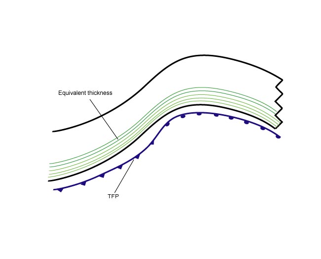
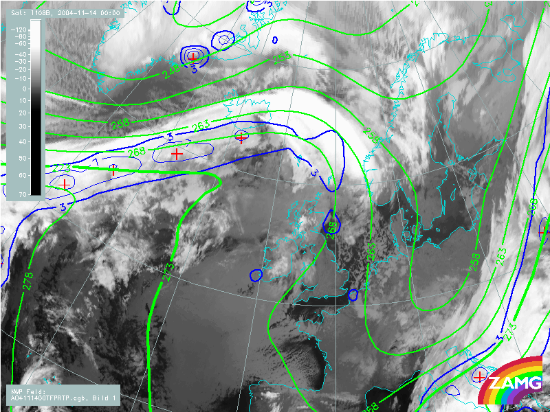
- Equivalent thickness:
The cloud band of the Warm Front Band is within the higher gradient zone of equivalent thickness. - Thermal front parameter (TFP):
The TFP can be found close to and parallel to the rear edge of the Warm Front cloud band. This is in contrast to the Ana Cold Front where the TFP accompanies the leading edge of the cloud band. - Warm advection (WA):
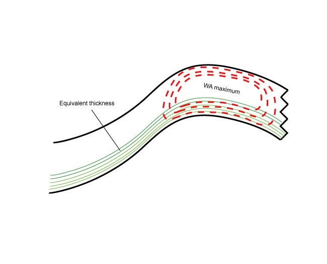
The whole frontal cloudiness lies within a WA maximum, which increases towards the occlusion point. Consequently, the maximum is in front of the frontal line. - Shear vorticity at 300 hPa:
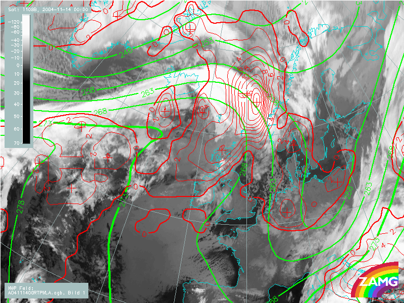
The zero line coincides with the leading edge of the Warm Front cloud band. - Isotachs at 300 hPa:
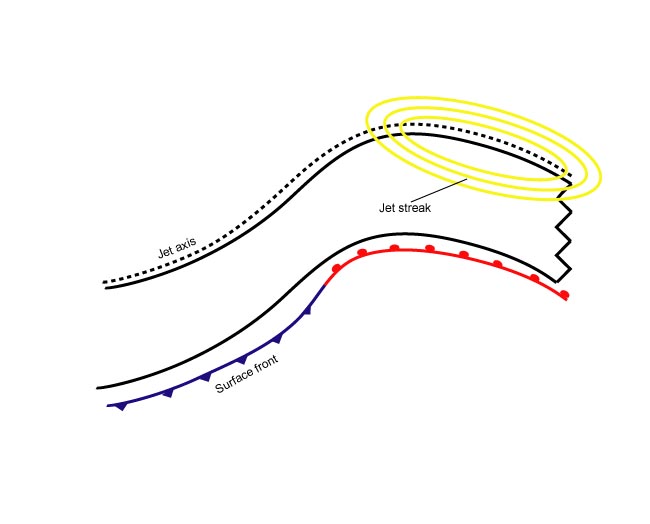
The leading edge of the Warm Front is superimposed upon a jet streak.
|
14 November 2004/00.00 UTC - Meteosat 8 IR 10.8 image; thermal front parameter (TFP) 500/850 hPa, green: equivalent thickness 500/850 hPa
|
|
|
|
|
14 November 2004/00.00 UTC - Meteosat 8 IR 10.8 image; red: temperature advection 500/1000 hPa, green: equivalent thickness 500/850 hPa
|
|
|
|
|
14 November 2004/00.00 UTC - Meteosat 8 IR 10.8 image; yellow: isotachs 300 hPa, black: zero line of shear vorticity 300 hPa
|
|
|
|
Typical Appearance In Vertical Cross Sections
The isentropes of the equivalent potential temperature across the Warm Front Band show a higher gradient zone through the whole troposphere which, looking downstream, is inclined from low to high levels. The colder air can be found in front of, and below, the warmer air in front of and above the gradient zone. (see Weather Events).
The field of humidity shows high values immediately behind and above the frontal surface of the Warm Front. Low values can be found below the gradient zone of the equivalent potential temperature.
Like the distribution of humidity, the field of temperature advection can also be separated into two parts. Therefore WA exists above and within the gradient zone of the Warm Front. The maximum of the WA can be found within the gradient zone in the mid-levels of the troposphere at approximately 500 hPa. On the other hand CA can be found below and in front of the gradient zone.
At the leading part above the frontal surface, at approximately 300 hPa, the atmosphere is characterized by a pronounced isotach maximum.
Well developed fronts are accompanied by a zone of distinct convergence within and divergence above the frontal zone. Consequently, upward vertical motion can be found above the frontal zone, responsible for cloud development.
The satellite images across the Warm Front are, in the ideal case, characterized by typical distributions. While across the frontal area the IR image shows continuously increasing values of grey shades from the rear to the leading edge, the distribution of grey shades in the VIS image is reversed (see Cloud Structure In Satellite Images). In contrast, the WV image shows high pixel values within the frontal cloudiness and a pronounced minimum associated with the dry air.
|
14 November 2004/00.00 UTC - Meteosat 8 IR 10.8 image; position of vertical cross section indicated
|
|
|
|
The first cross section shows the gradient zones of equivalent potential temperature of the surface and upper level warm front with intense WA within the whole troposphere. In the IR signal the sharp leading edge can be clearly discriminated. This decrease coincides with the decrease of the relative humidity field in the second cross section, while values higher than 80% mark out the frontal zones. The third cross section shows a zone of convergence within the lower level front, followed by intense upward motion within and above it. The fourth cross section finally shows the jet streak around 250 hPa and the associated, pronounced decrease of WV pixel values.
|
14 November 2004/00.00 UTC - Vertical cross section; black: isentropes (ThetaE), red thick: temperature advection - WA, red thin: temperature advection - CA, orange thin: IR pixel values, orange thick: WV pixel values
|
|
|
|
|
14 November 2004/00.00 UTC - Vertical cross section; black: isentropes (ThetaE), blue: relative humidity, orange thin: IR pixel values, orange thick: WV pixel values
|
|
|

|
|
14 November 2004/00.00 UTC - Vertical cross section; magenta thin: divergence, magenta thick: convergence, cyan thick: vertical motion (omega) - upward motion, cyan thin: vertical motion (omega) - downward motion, orange thin: IR pixel values, orange thick: WV pixel values
|
|

|

|
|
14 November 2004/00.00 UTC - Vertical cross section; black: isentropes (ThetaE), yellow: isotachs, orange thin: IR pixel values, orange thick: WV pixel values
|
|

|

|
Weather Events
Warm front bands are associated with multi-layered cloud structures, with clearances in the cloud-free regions in the warm sector. Precipitation can exist well ahead of the surface front, until just after the passage of the front.
| Parameter | Description |
| Precipitation |
|
| Temperature |
|
| Wind (incl. gusts) |
|
| Other relevant information |
|
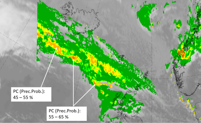
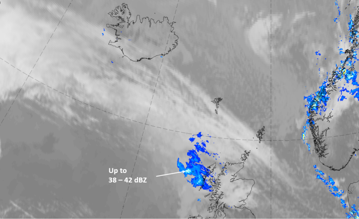
The case from 17 September 2019 at 12 UTC exists mostly over the sea but there are reports from some inhabited Islands which demonstrate the weather situation.
|
|
Legend:
17 September 2019 at 12UTC: IR + synoptic measurements (above) + probability of moderate rain (Precipitting clouds PC - NWCSAF).
Note: for a larger SYNOP image click this link.
There is no precipitation report from the existing weather stations (which are along the leading edge) but some spots with higher precipitation probabilities are at the rearward edge.
|
|
|
|
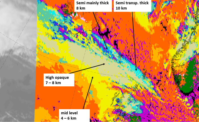
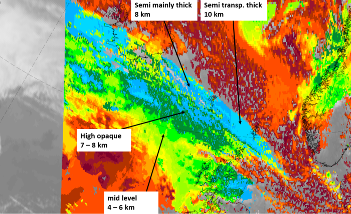
17 September 2019at 12 UTC
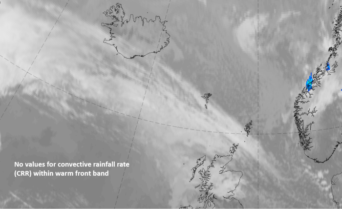
1st row: Cloud Type (CT NWCSAF) (above) + Cloud Top Height (CTTH - NWCSAF) (below); 2nd row: Convective Rainfall Rate (CRR NWCSAF) (above) + Radar intensities from Opera radar system (below).
For identifying values for Cloud type (CT), Cloud type height (CTTH), precipitating clouds (PC), and Opera radar for any pixel in the images look into the legends. (link).
References
General Meteorology and Basics
- BROWNING K. A. (1985): Conceptual models of precipitation systems; Quart. J. R. Meteor. Soc., Vol. 114, p. 293 - 319
- BROWNING K. A. (1986): Conceptual models of precipitation systems; Weather&Forecasting, Vol. 1, p. 23 - 41
- CONWAY B. J., GERARD L., LABROUSSE J., LILJAS E., SENESI S., SUNDE J. and ZWATZ-MEISE V. (1996): COST78 Meteorology - Nowcasting, a survey of current knowledge, techniques and practice - Phase 1 report; Office for official publications of the European Communities
- GREEN J. S. A., LUDLAM F. H. and MCILVEEN J. F. R. (1966): Isentropic relative-flow analysis and the parcel theory; Quart. J. R. Meteor. Soc., Vol. 92, p. 210 - 219
- HARROLD T. W. (1973): Mechanisms influencing the distribution of precipitation within baroclinic disturbances; Quart. J. R. Meteor. Soc., Vol. 99, p. 232 - 251
- HUBER-POCK F. and KRESS CH. (1989): An operational model of objective frontal analysis based on ECMWF products; Met. Atmos. Phys., Vol. 40, p. 170 - 180
- KURZ M. (1990): Synoptische Meteorologie - Leitfäden für die Ausbildung im Deutschen Wetterdienst; 2. Auflage, Selbstverlag des Deutschen Wetterdienstes
General Satellite Meteorology
- BADER M. J., FORBES G. S., GRANT J. R., LILLEY R. B. E. and WATERS A. J. (1995): Images in weather forecasting - A practical guide for interpreting satellite and radar imagery; Cambridge University Press
- CARLSON T. N. (1987): Cloud configuration in relation to relative isentropic motion; in: Satellite and radar imagery interpretation, preprints for a workshop on satellite and radar imagery interpretation - Meteorological Office College, Shinfield Park, Reading, Berkshire, England, 20 - 24 July 1987, p. 43 - 61
- ZWATZ-MEISE V. (1987): Satellitenmeteorologie; Springer Verlag, Berlin - Heidelberg - New York - London - Paris - Tokyo
Specific Satellite Meteorology
- BENNETTS D. A., GRANT J. R. and MCCALLUM E. (1988): An introductory review of fronts. Part I: Theory and observations; Met. Mag., Vol. 117, p. 357 - 370
- BENNETTS D. A., GRANT J. R. and MCCALLUM E. (1989): An introductory review of fronts. Part II: A case study; Met. Mag., Vol. 118, p. 8 - 12
- CARLSON T. N. (1980): Airflow through mid-latitude cyclones and the comma cloud pattern; Mon. Wea. Rev., Vol. 108, p. 1498 - 1509
- HERZEGH P. H. and HOBBS P. V. (1980): The mesoscale and microscale structure and organization of clouds and precipitation in mid-latitude cyclones. Part II: Warm front clouds; J. Atmos. Sci., Vol. 37, p. 597 - 611
- HOSKINS B. J. and HECKLEY W. A. (1981): Cold and warm fronts in baroclinic waves; Quart. J. R. Meteor. Soc., Vol. 107, p. 79 - 90
- HOUZE R. A. JR., RUTLEDGE S. A. and HOBBS P. V. (1981): The mesoscale and microscale structure and organization of clouds and precipitation in mid-latitude cyclones. Part III: Air motions and precipitation growth in a warm frontal rain band; J. Atmos. Sci., Vol. 38, p. 639 - 649
- LOCATELLI J. D. and HOBBS P. V. (1987): The mesoscale and microscale structure and organization of clouds and precipitation in mid-latitude cyclones. Part XIII: Structure of a warm front; J. Atmos. Sci., Vol. 44, p. 2990 - 2309
- RUTLEDGE S. A. and HOBBS P. V. (1983): The mesoscale and microscale structure and organization of clouds and precipitation in mid-latitude cyclones. Part VIII: A model for the "seeder - feeder" process in warm frontal rain bands; J. Atmos. Sci., Vol. 40, p. 1185 - 1206
- ZWATZ-MEISE V. (1990): Satellite synoptic of warm fronts; Proceedings of 8th Meteosat Scientific Users' meeting, Norrköping, Sweden, 28 - 31 August 1990, p. 151 - 160
Special Investigation:
•Different Kinds of Warm Front Development
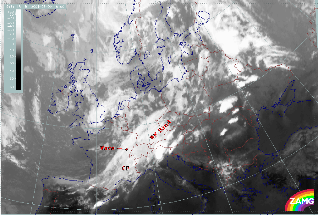
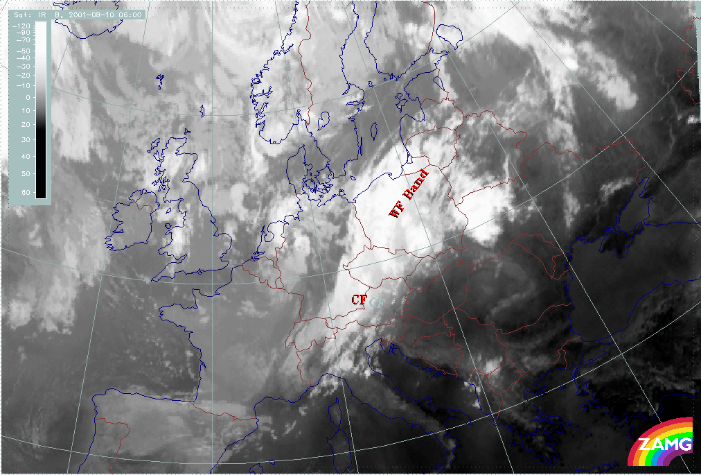
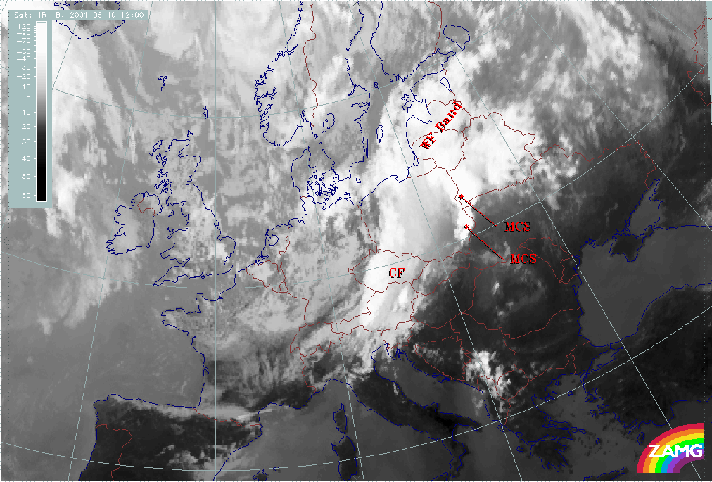
Warm Front Bands are described in this chapter as CMs standing alone. But it is especially interesting to look at the development of such weather systems.
The most common development of a Warm Front Band is connected to classical Norwegian Model of the polar front theory; that means that Cold Fronts and Warm Fronts develop if a disturbance is superimposed on the (in the beginning stationary) polar front (see also Occlusion: Warm Conveyor Belt Type).
|
|
|
|
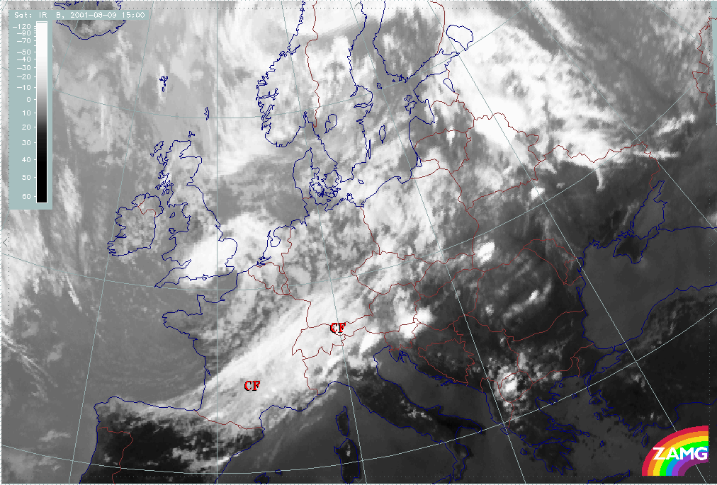
09 August 2001/15.00 UTC - Meteosat IR image
|
09 August 2001/18.00 UTC - Meteosat IR image
|
|
|
|
|
|
10 August 2001/06.00 UTC - Meteosat IR image
|
10 August 2001/12.00 UTC - Meteosat IR image
|
There are two examples in the "Case Study" part of this manual:
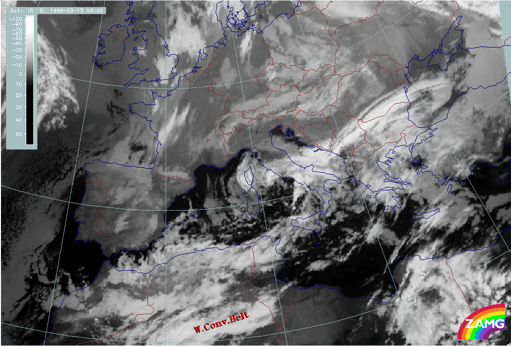
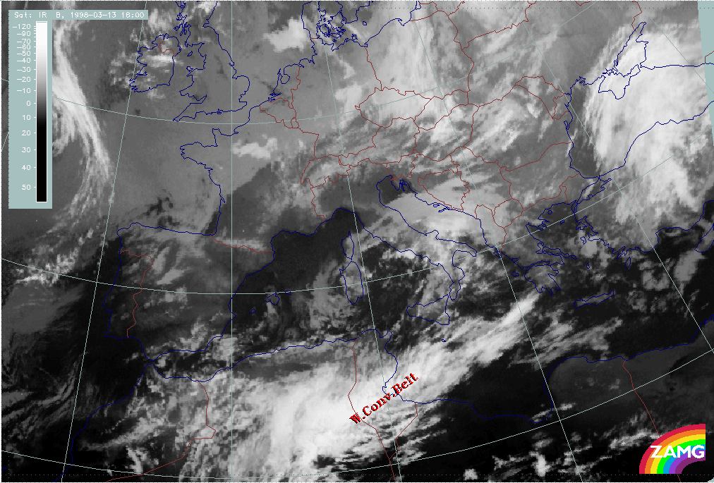
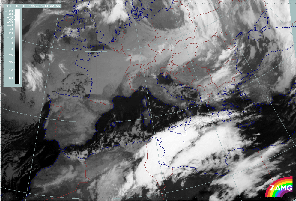
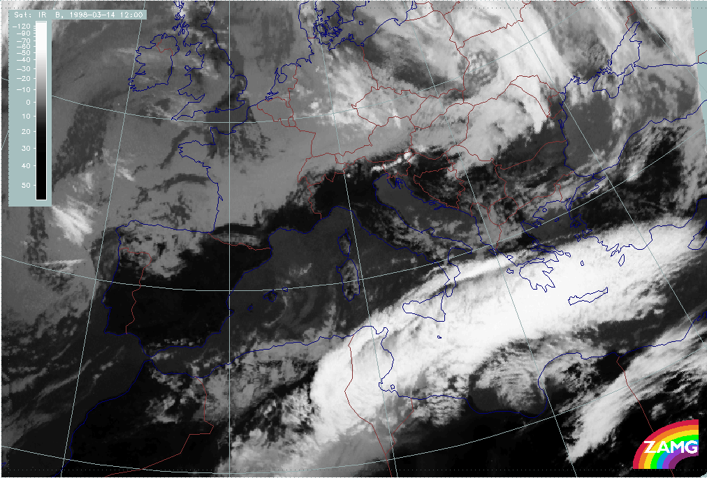
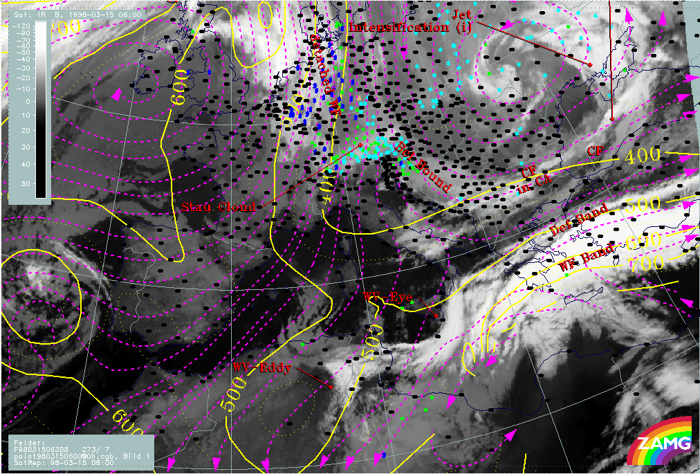
1. The case from 13 - 15 March 1998 which shows the development of a very pronounced Warm Front cloud band over the Eastern Mediterranean/Turkey. Its initial stages can be followed backwards to the Sahara where cloudiness in the typical form of a Warm Conveyor Belt can be observed.
|
13 March 2001/06.00 UTC - Meteosat IR image
|
13 March 2001/18.00 UTC - Meteosat IR image
|
|
|
|
|
|
14 March 2001/06.00 UTC - Meteosat IR image
|
14 March 2001/12.00 UTC - Meteosat IR image
|
|
15 March 1998/06 UTC - IR image; SatRep overlay: names of conceptual models; symbols: weather events (green: rain and showers, blue: drizzle, cyan: snow, purple: freezing rain, red: thunderstorm with precipitation, orange: hail, yellow: fog, black: no actual precipitation or thunderstorm with precipitation); lines: magenta: relative streams on 308 K, yellow: isobars, system velocity 273? 7 m/s
|
|
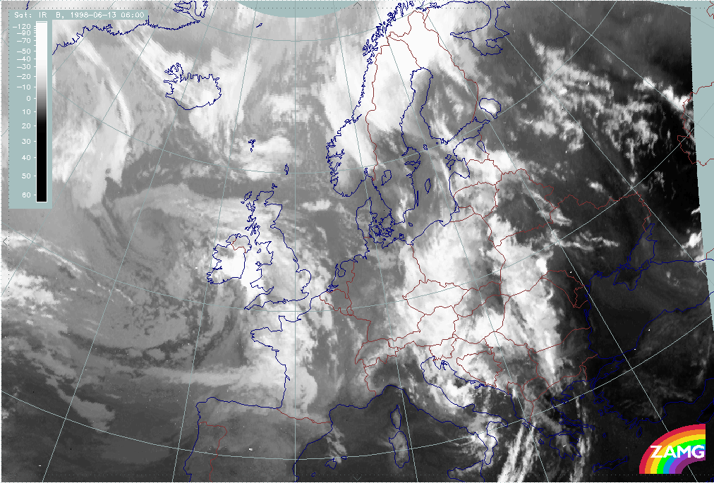
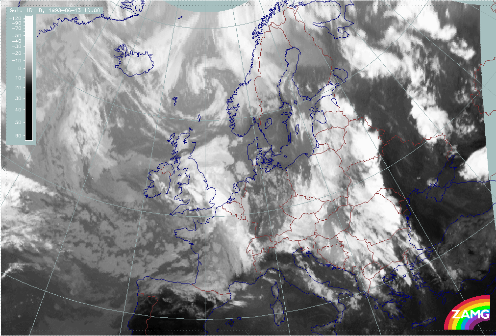
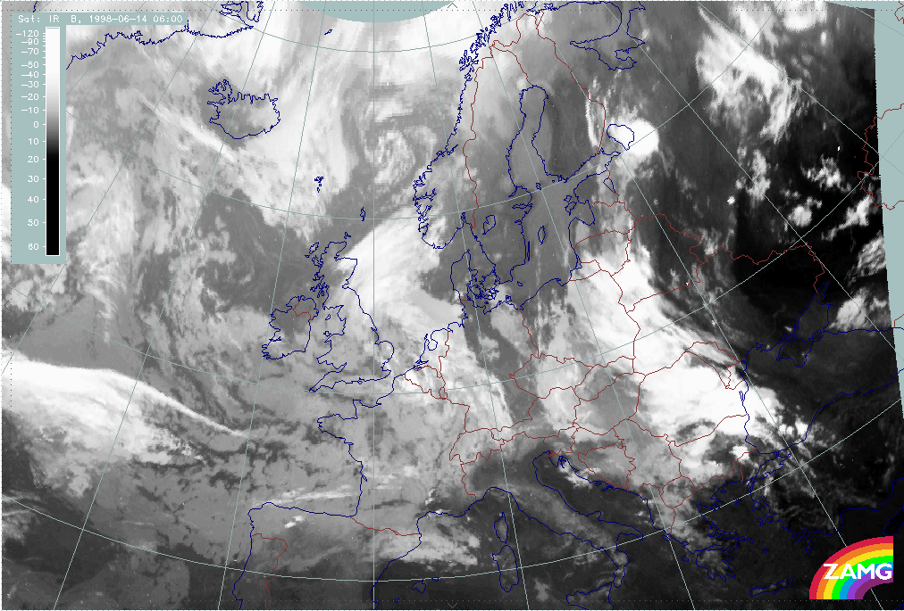
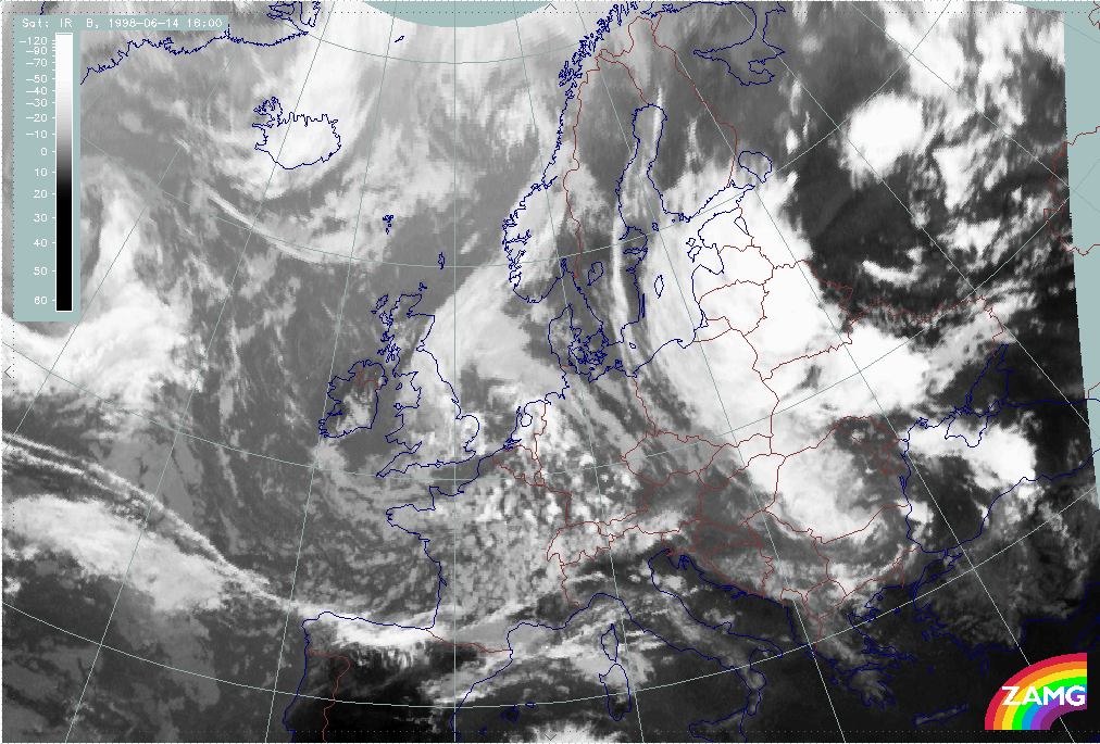
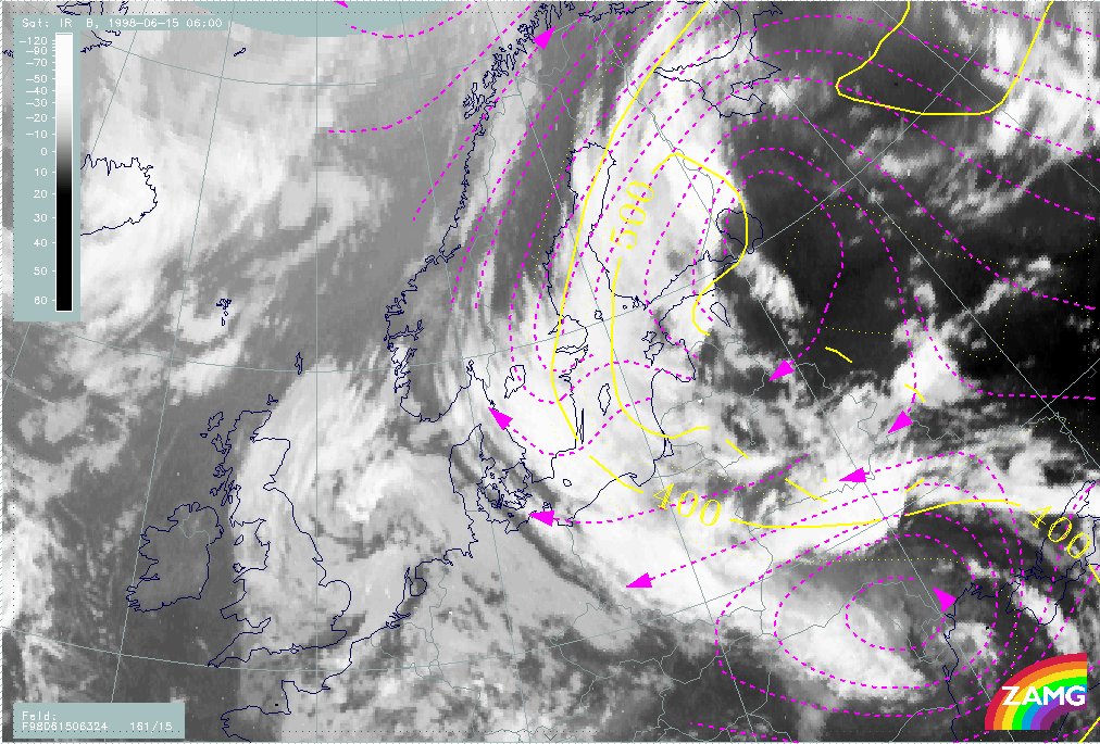
2. The case from 14 - 15 June 1998 (see Case Study 14 - 15 June 1998 ) which shows a Warm Front cloud band moving from SE Europe across Finland and the Scandinavian countries westward. The initial stages of cloudiness can be found over the Balkan Peninsula within a warm air mass.
|
13 June 1998/06.00 UTC - Meteosat IR image
|
13 June 1998/18.00 UTC - Meteosat IR image
|
|
|
|
|
|
14 June 1998/06.00 UTC - Meteosat IR image
|
14 June 1998/12.00 UTC - Meteosat IR image
|
|
15 June 1998/06 UTC - IR image; isobars (yellow) and relative streams (magenta) on 324K
|
|