Rapid Cyclogenesis

Cloud Structure In Satellite Images

Appearance in the basic channels

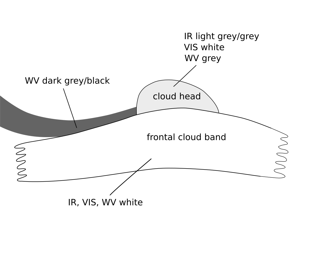
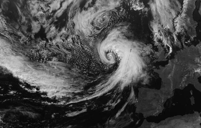
IR10.8 imagery:

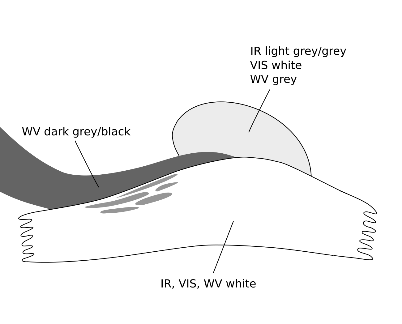
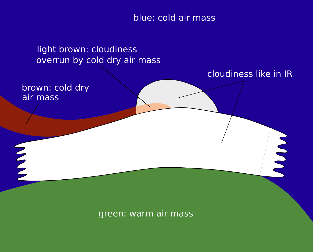
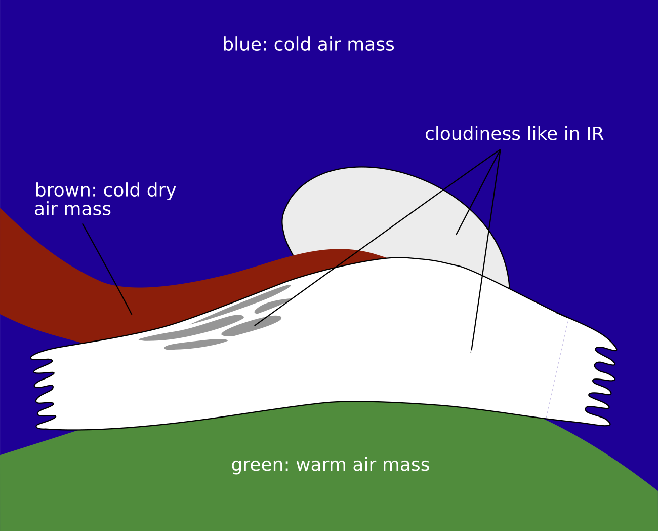
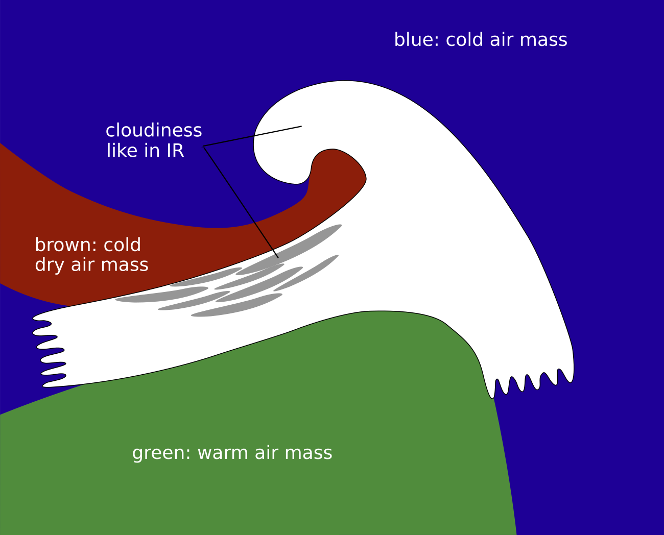
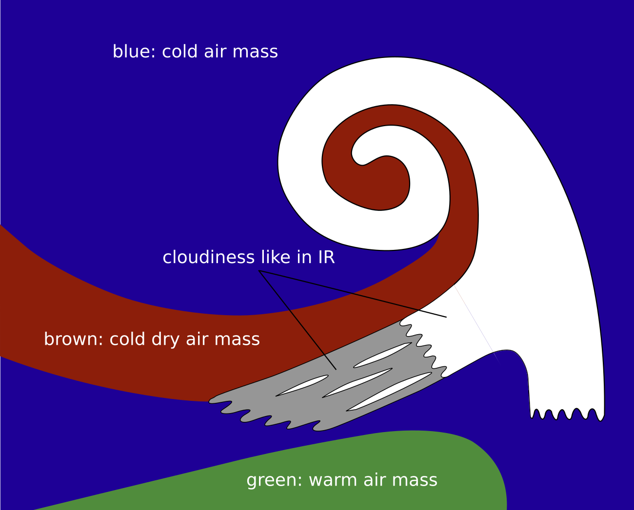
• Two main cloud configurations are seen during the initial stages of a rapid cyclogenesis: a frontal cloud band usually oriented east to west and clouds with warmer tops that form an increasingly dense shield, a so-called "cloud head", on the poleward side of the frontal cloud band and protruding from below it. The developing cloud head varies between grey and light grey in the IR channels, mostly with higher tops on the poleward side.
• Dry sinking air originating from the lower levels of the stratosphere on the cyclonic side of a jet stream is advected downstream. This leads to a dark, cloud-free area between the cloud band of the cold front and the cloud head, thereby creating a V-pattern (often also called a dry slot).
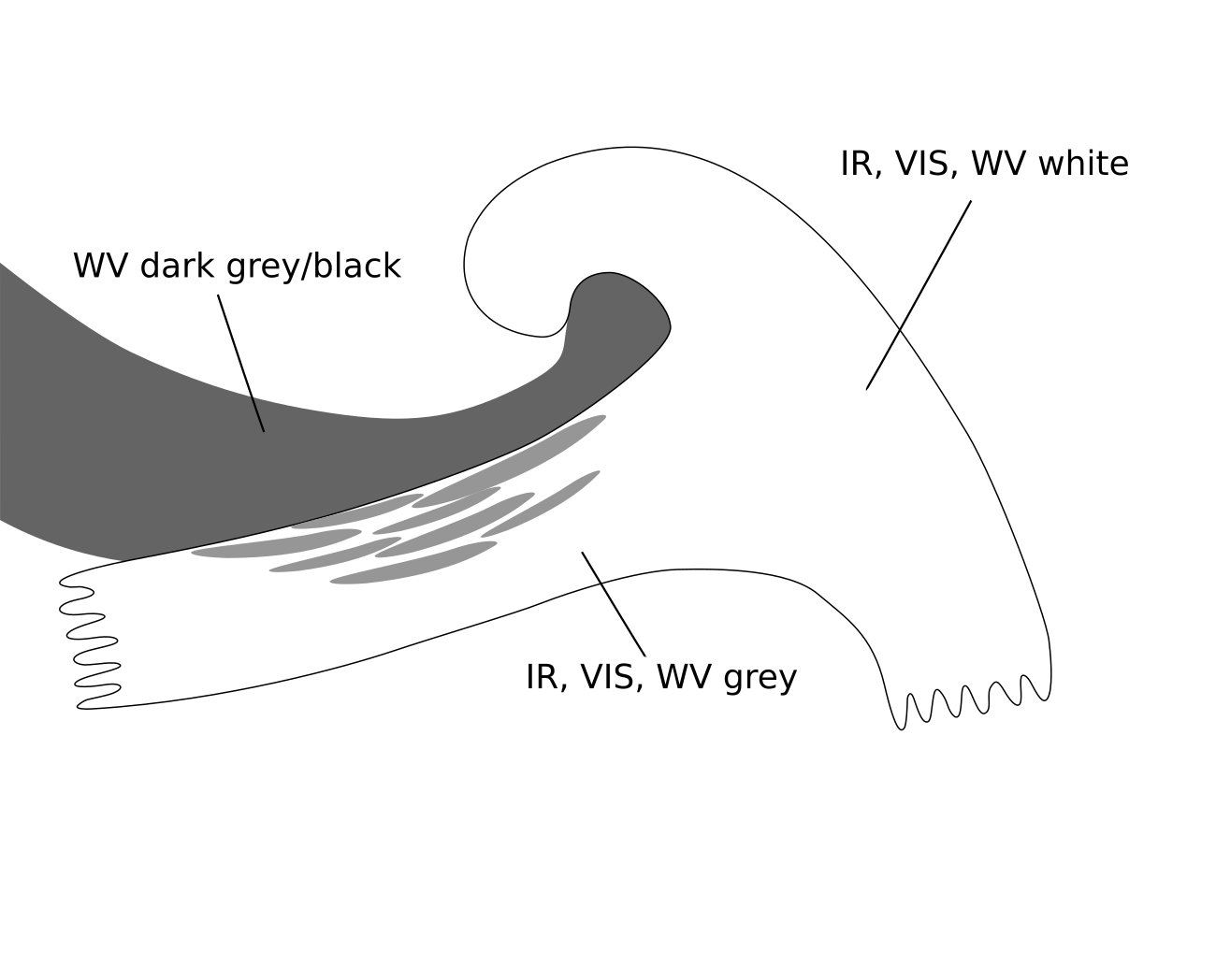
• During the advanced stages the cloud head grows to a cyclonically curved cloud spiral with a broad dark area between the spiral and the frontal cloud band; additionally, the rear part of the cold frontal cloud frequently dissolves as a consequence of sinking dry air.
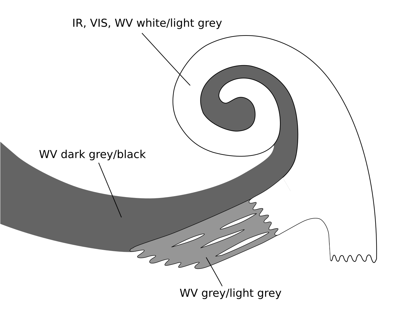
• Further development leading to the mature stage of the cyclone often includes a cloud spiral around the low centre.

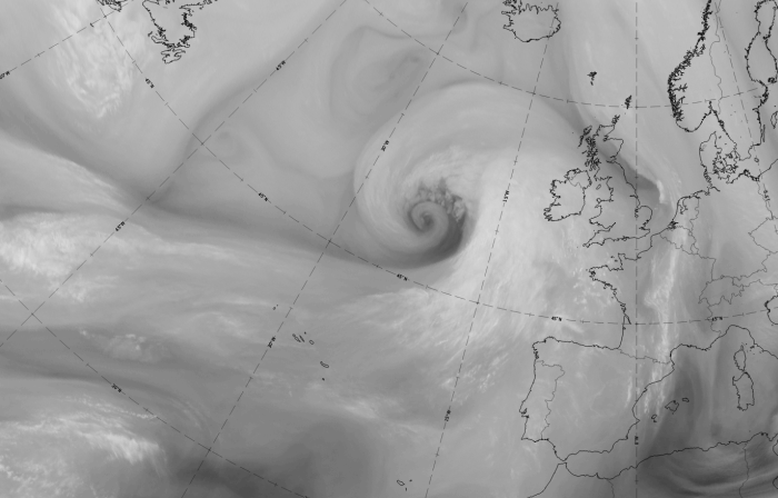
WV6.2 imagery:

• WV images have an important role in identifying the possibility of rapid cyclogenesis initiation.
• In the initial stage of the development a dark grey stripe can be seen along the northward edge of the white frontal cloud band. This stripe represents dry air sinking from the stratosphere along the cyclonic side of a jet stream.
• Before the development starts, the dark grey stripe is more distinct upstream of the cloud head.
• In the next stage the dark grey stripe approaches the cloud head while becoming darker and darker (indicating dry air moving downwards in the upper troposphere) and finally forming a typical V-pattern together with the cloud head.
• During the advanced stages the cloud head grows into a cyclonically curved cloud spiral with a broad black area between the spiral and the frontal cloud band.
• A further dark stripe often develops along the north- to north-eastern boundary of the cloud head in the cold air region within the cold airmass, indicating sinking movement. This is in connection with a second jet streak which often develops there.

VIS0.6 imagery:

• During their initial stages both the west-to-east oriented frontal cloud band as well as the cloud head appear white in the VIS image, indicating fairly thick cloud depth.The clouds have an irregular structure and sometimes fibrous edges on the poleward edge of the frontal cloud band.
• As the top of the frontal cloud band is higher than that of the cloud head, the frontal clouds can cast a distinct shadow on the cloud head, which is visible in VIS images.

Legend:
Schematics for the stages of Rapid Cyclogenesis seen through the basic channels IR, WV and VIS
ul.: initial stage; ur.: development stage; ll.: advanced stage; lr.: mature stage.
*Note: click on the image to access the image gallery (navigate using arrows on keyboard)

Appearance in the basic RGBs:

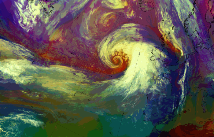
Airmass RGB

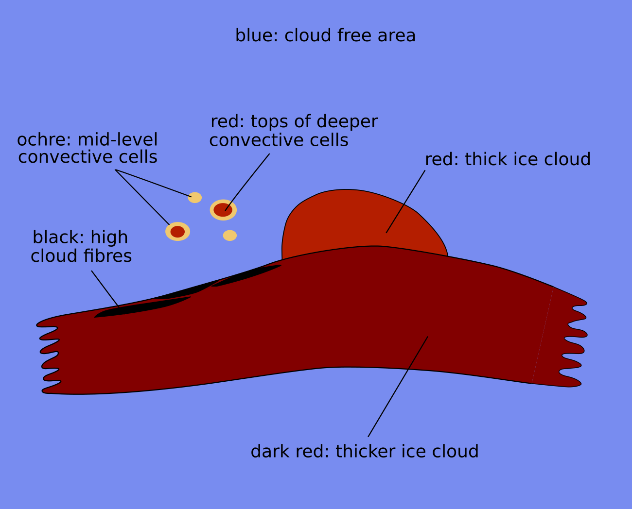
The most important feature in an airmass RGB during the whole development is the dark-brown stripe along and at the rear of the frontal cloud band; it is indicative of the sinking cold and dry stratospheric air. Typically, in the initial phase there is mostly only a stripe extending from west to northwest, towards the rearward edge of the cloud head. As the development continues the stripe broadens and intensifies into a distinct V-pattern between the cloud head and the frontal cloud band. Finally, during the advanced stage, the V-pattern transitions into a circular hole area in the centre of the developing cloud spiral. This development makes the acceleration of the rapid cyclogenesis clearly visible. From the advanced to the mature stage, very intensive dark-brown colours fill the whole area within the spiral.

The clouds look very similar in the IR images. Sometimes, in the initial stage, the southern part of the cloud head is overrun by dry air which results in some brownish shadows there.

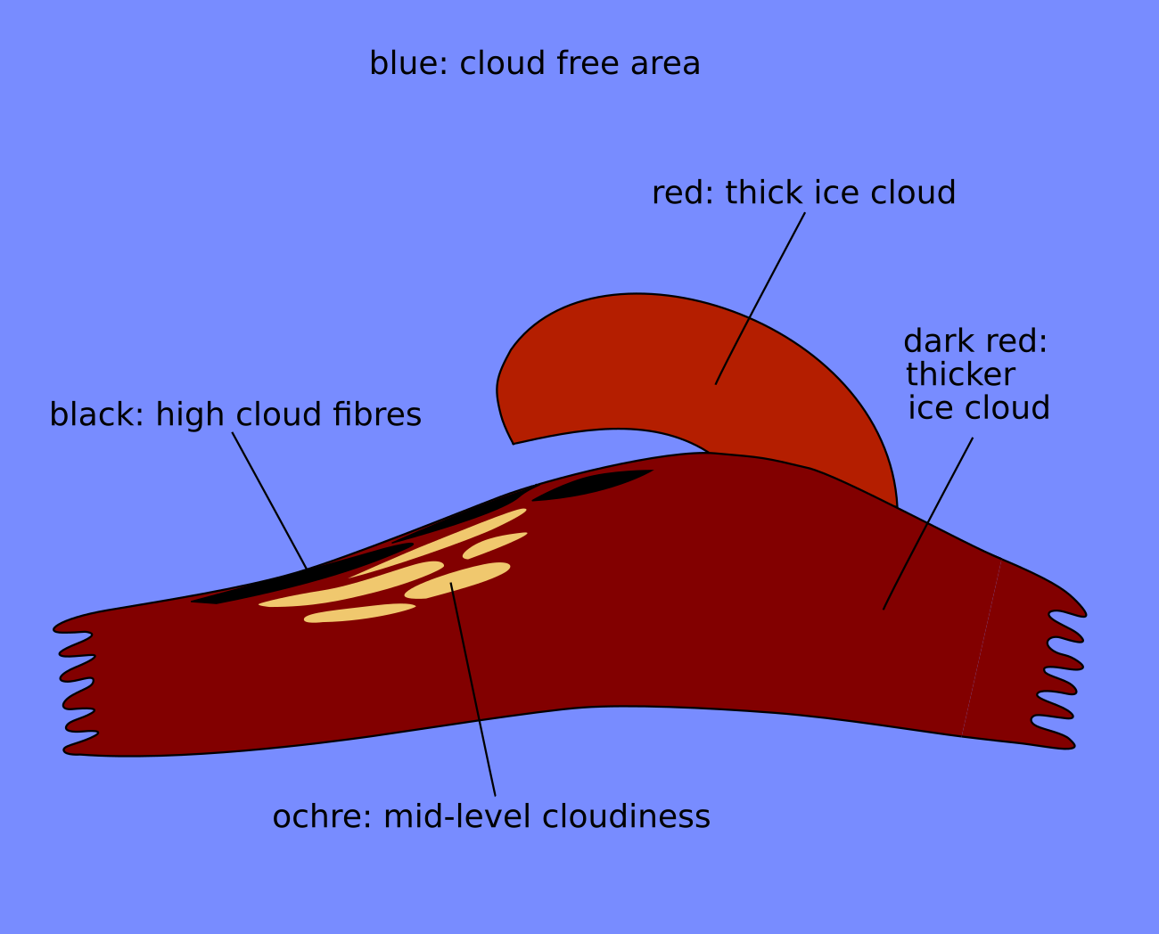
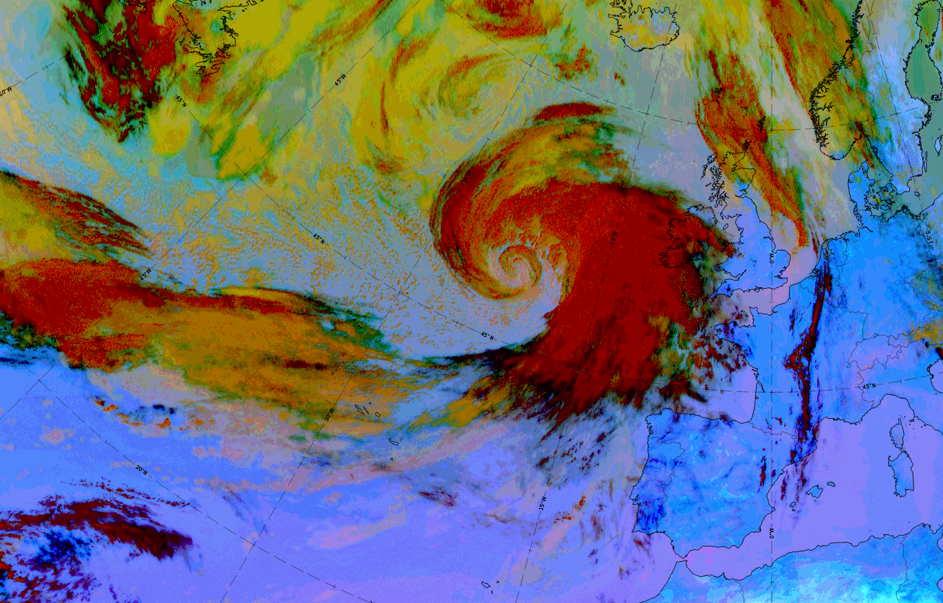
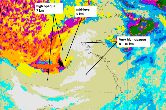
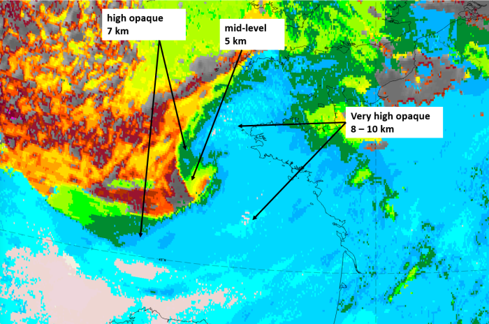
Dust RGB

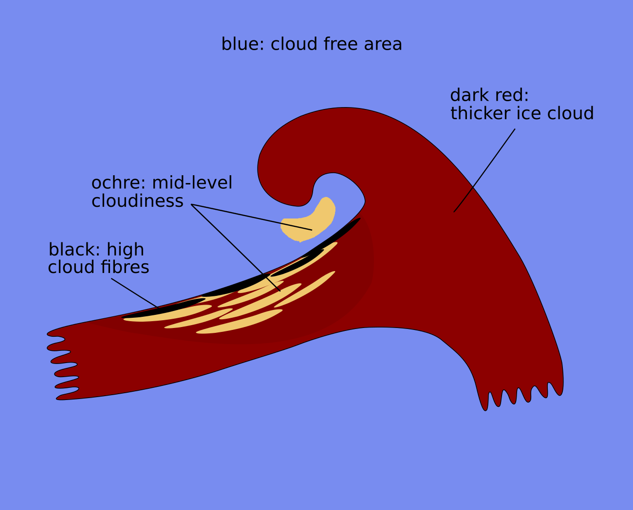
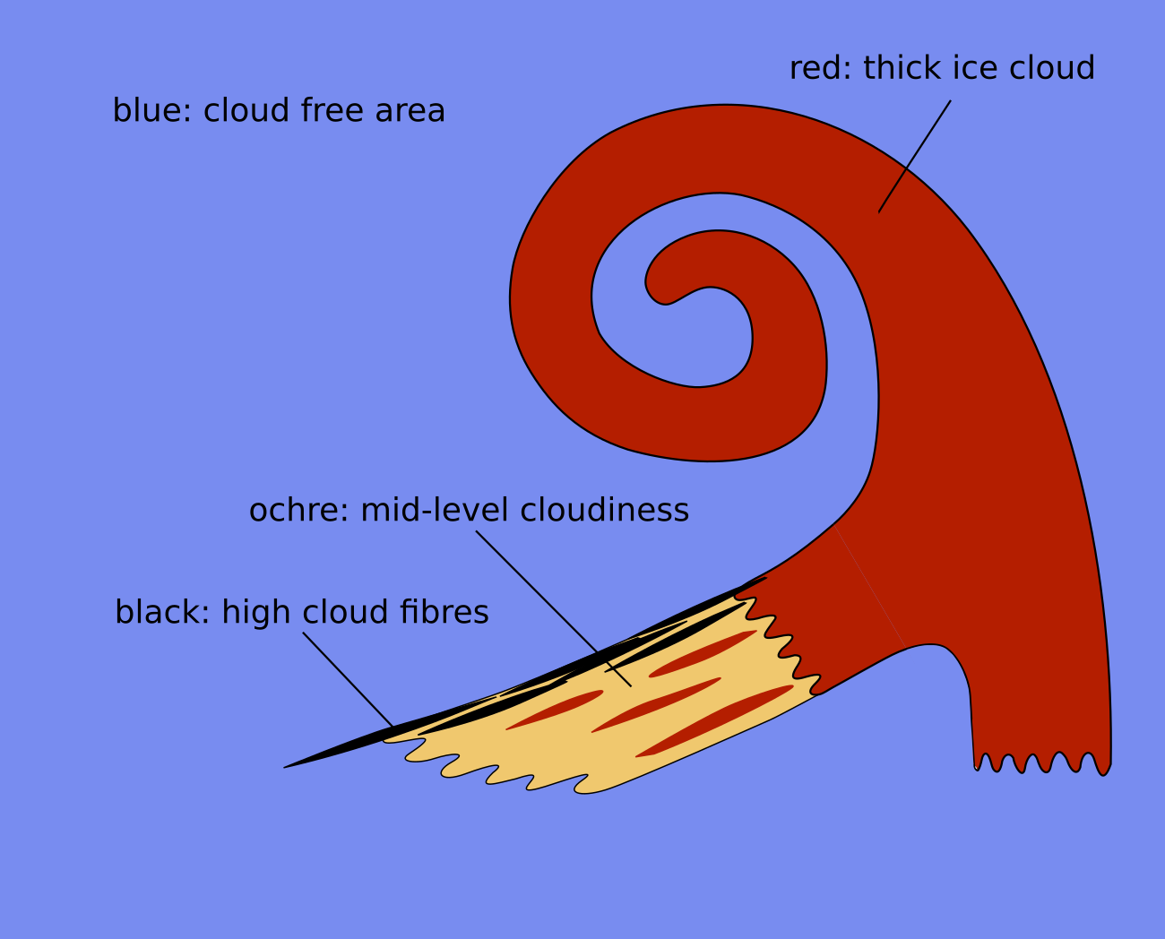
The surroundings of the cloud system undergoing rapid cyclogenesis have blue colours in all development stages. In these locations which only differs if thin low or mid-level clouds exist-indicated by ochre or green cloud patches.

In the initial stage, the cloud head which appears in the IR images is less bright and colder than the frontal cloud as seen in the dust RGB. If visible, only small differences exist between the two cloud systems. Both parts consist of thick ice cloud. However, a dissolution of the clouds in the frontal cloud band can often be observed by the development of ochre colours. In those cases, a black cloud fibre remains at the northern boundary of the frontal cloud band where the jet axis is located. In advanced and mature stage later on, the cloud spiral appears dark-red due to the thick ice cloud.

Legend:
Schematics of basic RGBs; initial phase
left: airmass; right: dust.

Legend:
Schematics of basic RGBs; development phase
left: airmass; right: dust.

Legend:
Schematics of basic RGBs; advanced phase
left: airmass; right: dust.

Legend:
Schematics of basic RGBs; mature phase
left: airmass; right: dust.

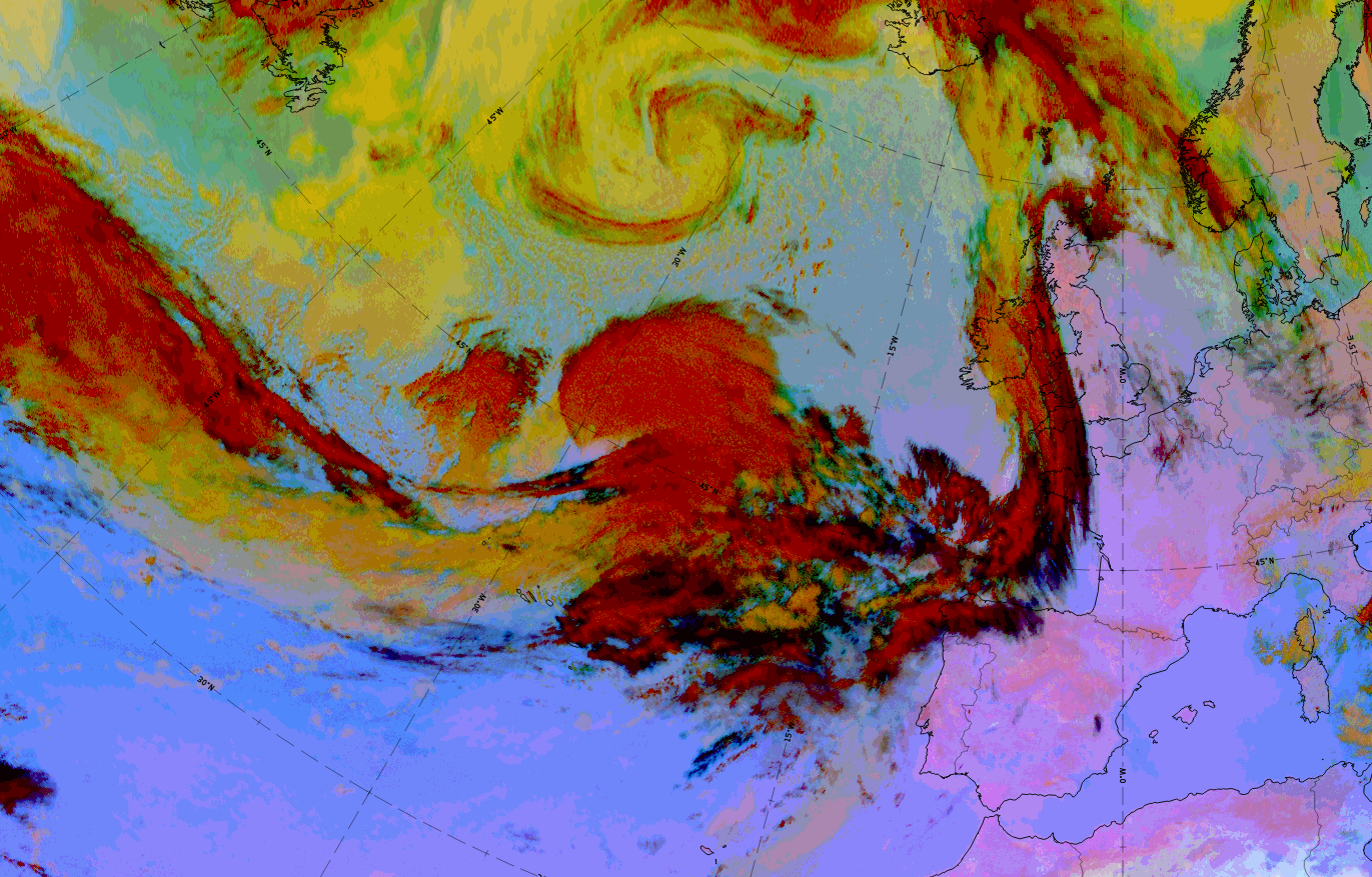
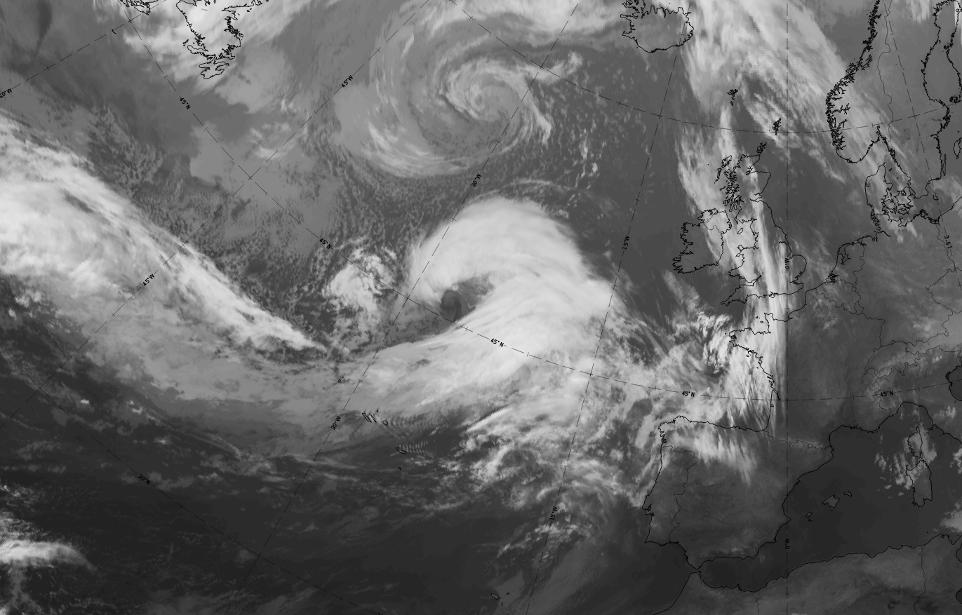
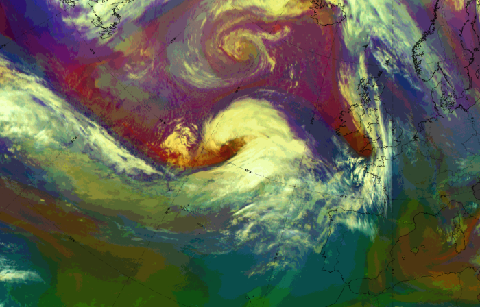
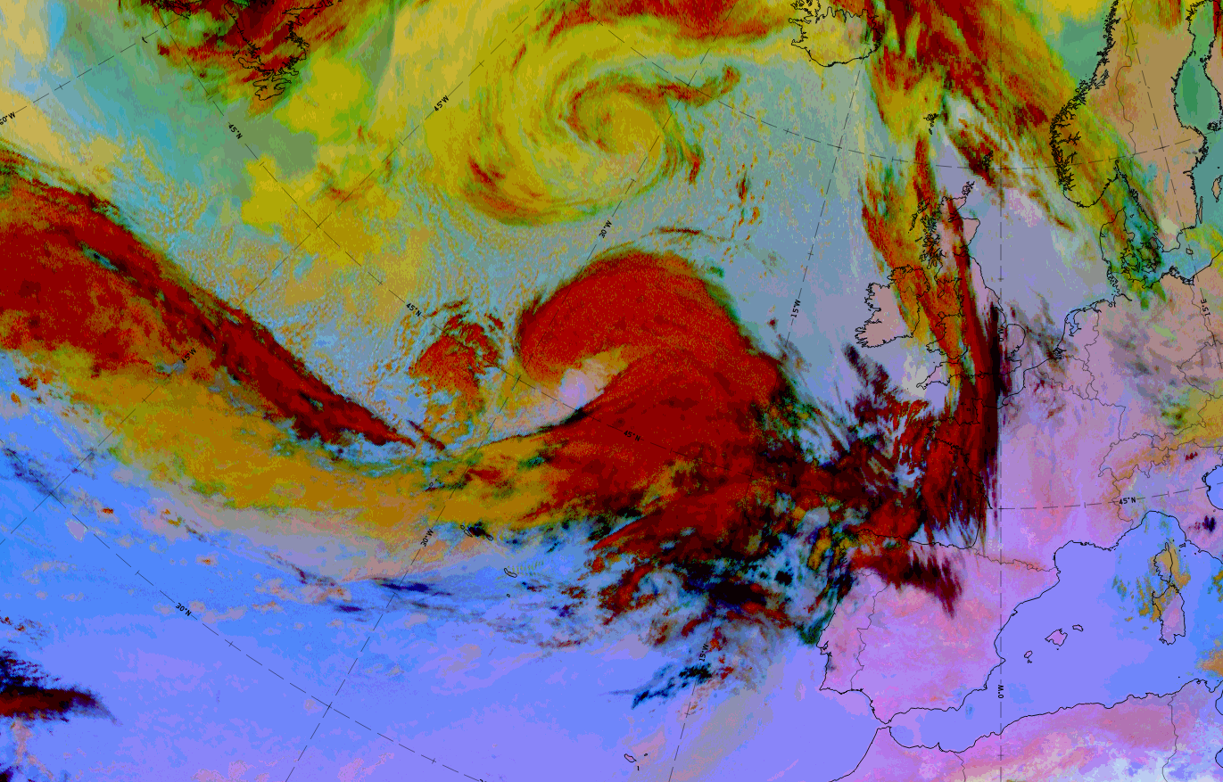
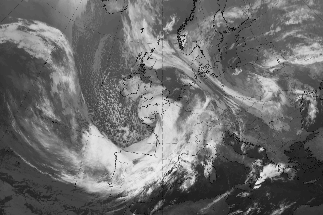
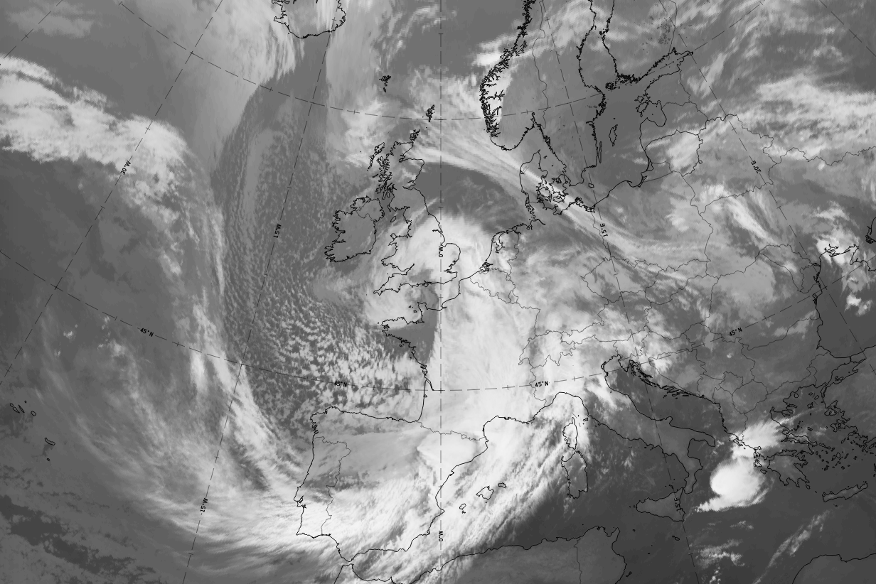
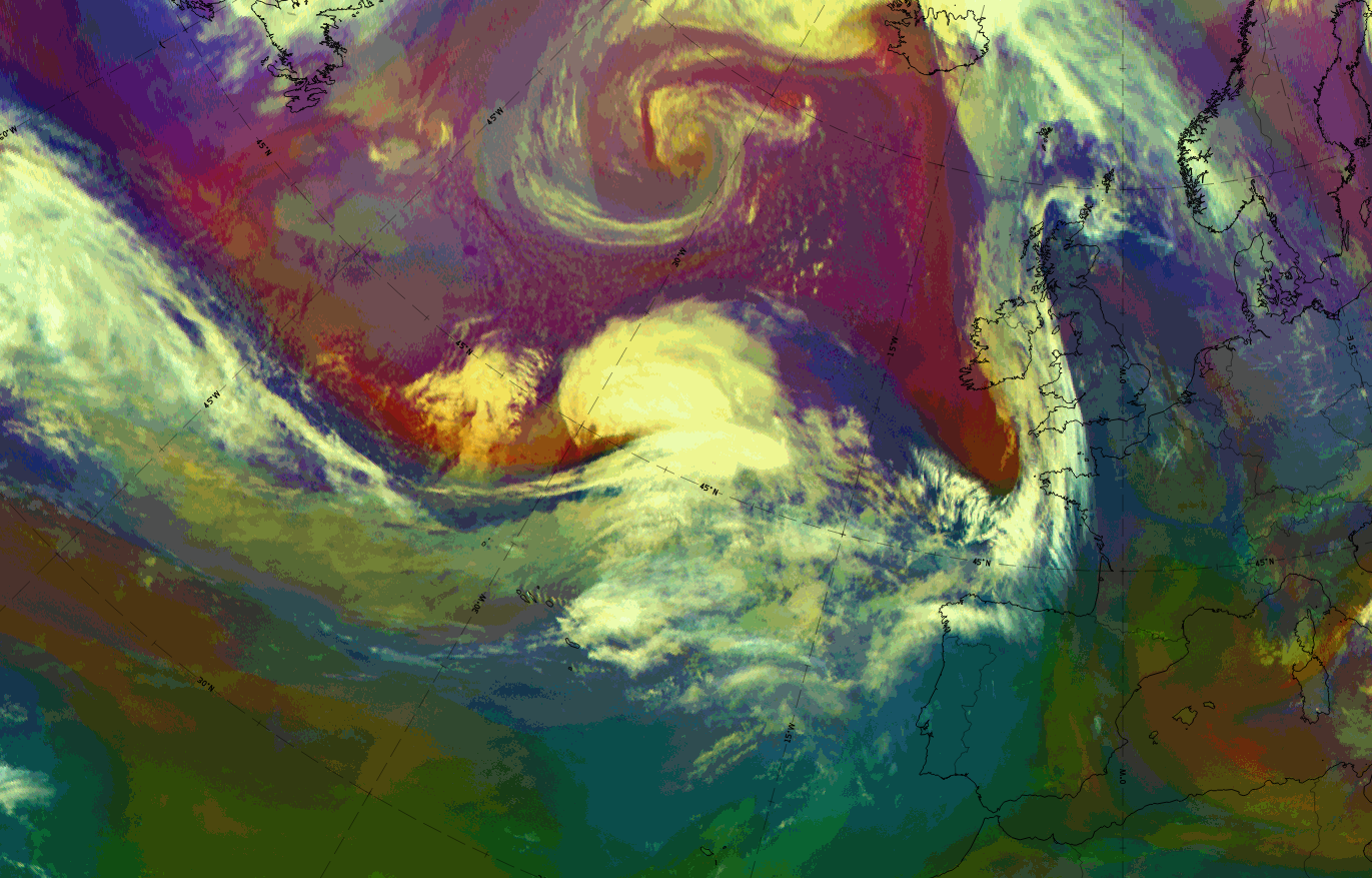
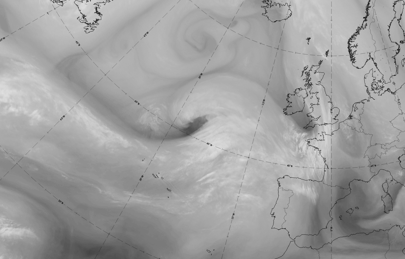
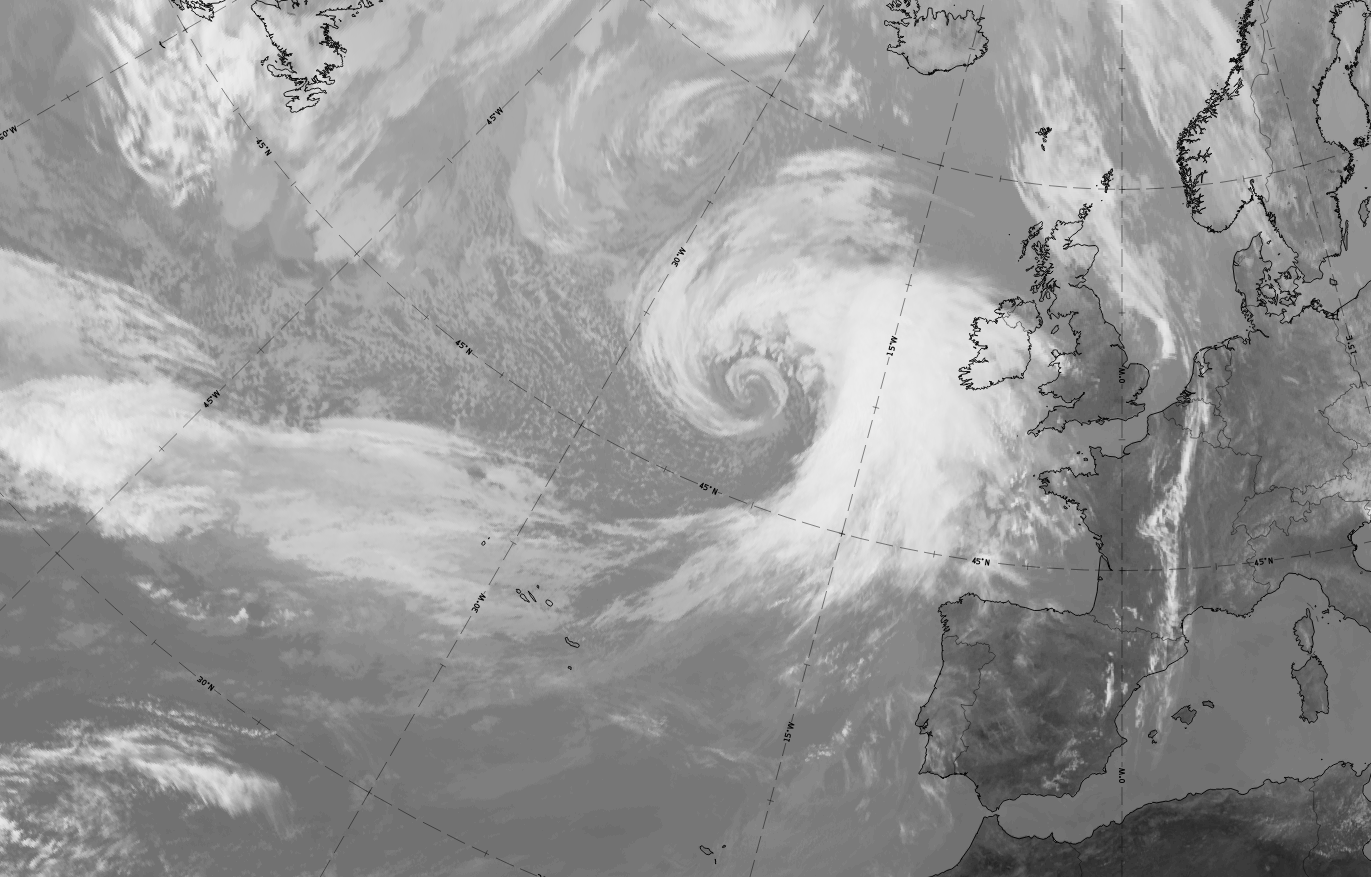
The case of 20 - 21 May 2020 is a clear example which shows all of the development stages of a Rapid Cyclogenesis very well. The development takes place in the Atlantic, starting from approximately 45 N, 30 W moving on a slightly north-westward path towards the British Isles. The rapid development takes place from 20 May 18 to 21 May 06 UTC with a central pressure drop of 25 hPa at the 1000 hPa level. In the initial and development stages there is a comma-like cloud feature to the west of the cloud head. Note that the comma-like cloud is a speciality of this case that does not belong to the rapid cyclogenesis development and dissolves during the whole process.

Rapid cyclogenesis: initial stage

Legend:
20 May 2020, 12UTC: initial stage
1st row: IR (above) + HRV (below); 2nd row: WV (above) + Airmass RGB (below); 3rd row: Dust RGB + image gallery.
*Note: click on the image to access the image gallery (navigate using arrows on keyboard)

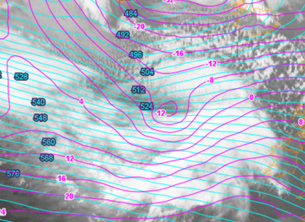
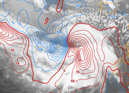
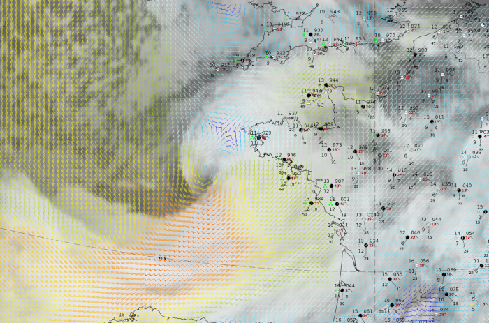
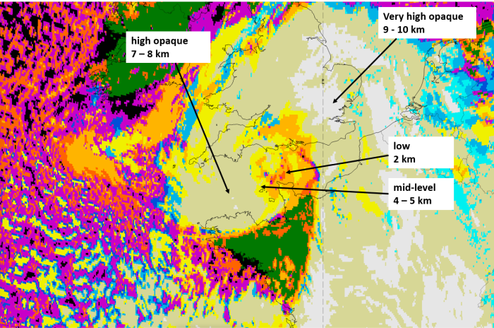
IR	Cloud head very bright; frontal cloud band dark grey; bright fibre at jet axis oriented from west to east.
HRV	Cloud head very bright; frontal cloud band grey; grey cloud fibre at jet axis oriented from west to east.
WV	Cloud head light grey; dark stripe from west to east ending at the western boundary of the cloud head. This represents the approaching, sinking, dry stratospheric air.
Airmass RGB	Broad blue band in the area of the frontal cloud band represents the cold air mass; a dark-brown stripe to the north extending from west to the western edge of the cloud head indicates the sinking, dry stratospheric air.
Dust RGB	Dark-red colours for the cloud head; ochre colours for the frontal cloud band; and dark-red to black colours for the fibres at the jet axis.
General remark	In this case the first two stages deviate from the schematics which show the usual situation. The cloud head amount is more intensive than the frontal cloud amount which highlights an exceptionally strong rising relative stream in the area of the cloud head, and only a weak warm conveyor belt in the area of the cold front band.

Rapid cyclogenesis: development stage

*Note: click on the image to access the image gallery (navigate using arrows on keyboard)

Legend:
21 May 2020, 00UTC: development stage
1st row: IR; 2nd row: WV (above) + Airmass RGB (below); 3rd row: Dust RGB + image gallery.
*Note: click on the image to access the image gallery (navigate using arrows on keyboard)

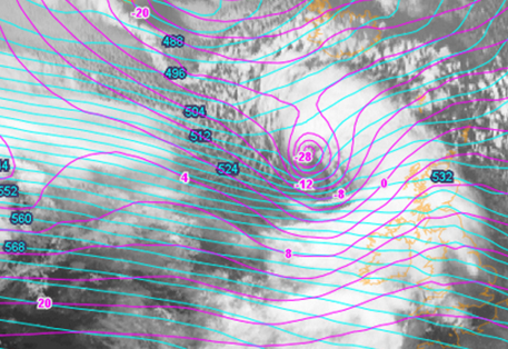
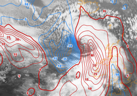
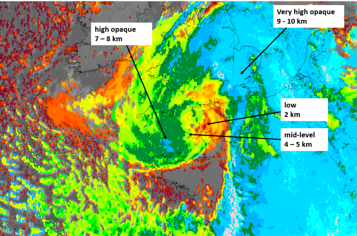
IR	Cloud head and eastern part of cold front are very bright; a bright fibre at the jet axis is oriented from west to east. Most important feature: a black V-pattern between cloud head and the frontal cloud band, indicating the start of the rapid deepening of the low pressure.
HRV	Not available.
WV	Cloud head and eastern part of cold front are very bright; black stripe to the north of the cloud band ends in the V-pattern between the cloud head and the cold front, and indicates the east-ward protrusion of the dry stratospheric air.
Airmass RGB	Corresponding to the WV image, the dark-brown stripe ends in the V-pattern and indicates the east-ward protrusion of the dry stratospheric air.
Dust RGB	Dark-red colours for the cloud head; ochre colours for the frontal cloud band and dark-red to black colours for the fibre at the jet axis. The area in the V-pattern shows blue colours indicating the cloud free ground below, caused by the sinking air within the centre of the cyclonic circulation.

Rapid cyclogenesis: advanced stage

*Note: click on the image to access the image gallery (navigate using arrows on keyboard)

Legend:
21 May 2020, 03UTC: advanced stage
1st row: IR; 2nd row: WV (above) + Airmass RGB (below); 3rd row: Dust RGB + image gallery.
*Note: click on the image to access the image gallery (navigate using arrows on keyboard)

IR	Cloud spiral and eastern parts of the frontal cloud bands are very bright.
HRV	Not available.
WV	Whole frontal system is white to light grey. The black stripe at the northern edge of the cold front streams into a large black-coloured hole in the centre of the developing cloud spiral.
Airmass RGB	Corresponding with the WV image, the dark-brown stripe ends in the centre of the developing cloud spiral, indicating dry stratospheric air is sinking at the centre of the occlusion spiral.
Dust RGB	Dark-red colours in the cloud spiral of the cyclogenesis and the eastern parts of the frontal cloud bands; ochre colours for the western parts of the cold front cloud band and black colours for the fibre at the jet axis. The centre of the cloud spiral is partly blue where it is cloud free and partly ochre where there are low cloud patches.

Rapid cyclogenesis: mature stage

Legend:
21 May 2020, 12 UTC: mature stage
1st row: IR (above) + HRV (below); 2nd row: WV (above) + Airmass RGB (below); 3rd row: Dust RGB + image gallery.
*Note: click on the image to access the image gallery (navigate using arrows on keyboard)

IR	Developed cloud spiral and frontal cloud bands are very bright.
HRV	Developed cloud spiral and frontal cloud bands are very bright.
WV	Developed cloud spiral and frontal cloud bands are light grey to bright. Large dark grey to black area exists in the centre of the cloud spiral
Airmass RGB	Corresponding to the WV image, the dark-brown stripe ends in the centre of the developed cloud spiral and indicates the dry stratospheric air there.
Dust RGB	Dark-red colours for the cold and warm front system and for large areas in the occlusion spiral. Towards the centre of the spiral, ochre cloud areas become larger indicating the dissolution of the thicker cloud there. Other than some ochre cells in the cold air behind the frontal system, blue colours indicate cloud-free ground. The black fibres and areas at the south-western edge of the cold front band indicate thin, high-level ice cloud exist there.

Summarising, there are two major features of a rapid cyclogenesis seen in satellite images and image loops:

1. A mainly west to east oriented cold front-warm front cloud band together with a cloud head on the poleward side;
2. An approaching dark grey stripe in the WV image. As soon as the leading edge of this dark grey strip becomes darker and wider, close to the area between the cloud head and frontal cloud band, the rapid development will take place in just a few hours.

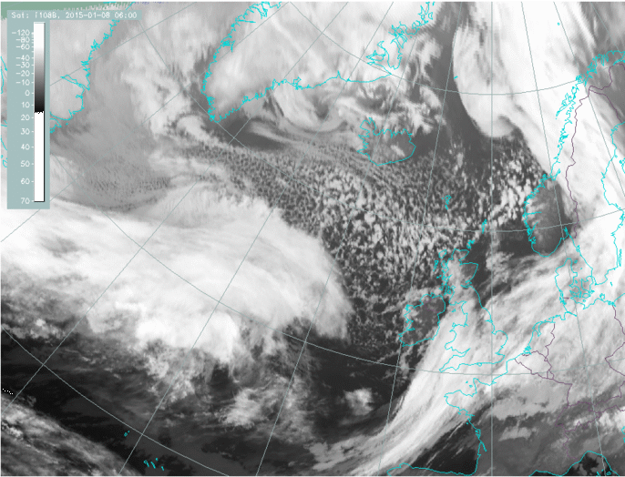
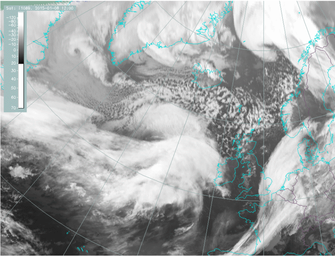
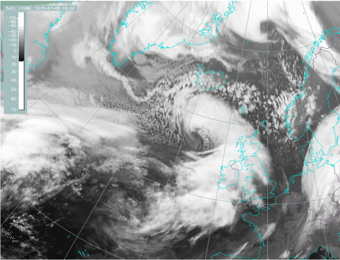
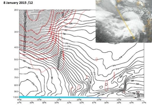
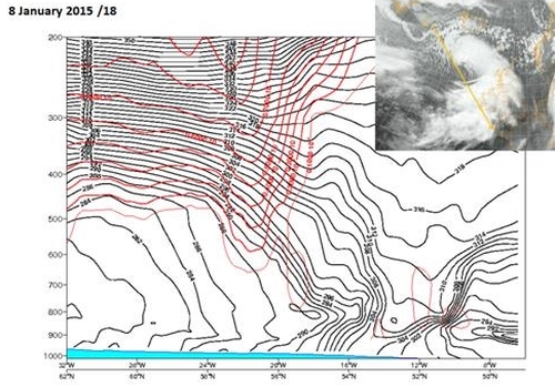
Another case used throughout all chapters of this conceptual model took place over the eastern Atlantic from 7 to 9 January 2015 and demonstrates the typical structures and the development of a typical rapid cyclogenesis. This case shows some features which are typical for a rapid cyclogenesis but cannot be observed distinctly in the case study above: a development loop, as well as the development of some small scale band features in the last stages.

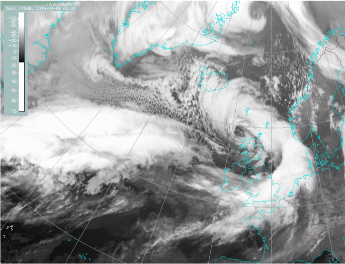Legend: 8-9 January 2015, IR images
u.l.: 8 January 06 UTC: initial stage; u.r.: 8 January 12 UTC: development stage; l.l.: 8 January 18 UTC: advanced stage; l.r.: 9 January 00 UTC: mature stage

In the advanced and mature stages, when the cloud spiral is well developed and circling the cyclone's centre, parallel cloud lines can appear close to the innermost part of the cloud spiral. These cloud bands are parallel rain bands. Although rain bands are by their nature more visible on radar than in satellite images, they are mentioned here because they can appear together with a very dangerous phenomenon, a sting jet. The sting jet will be described in more detail in the chapter on weather phenomena.

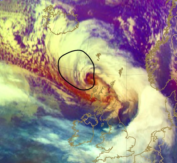
Fig. 9: 9 January 2015, 00 UTC, airmass. The black line encompasses an area of banded cloud which can be correlated to severe weather events in terms of wind and convection.
*Note: click on the image to access the image gallery (navigate using arrows on keyboard)

The following loops show a very rapid development of the depression over 12 hours from 990 hPa on 8 January 2015, 06 UTC to the extreme low value of 965 hPa on 8 January 2015, 18 UTC.

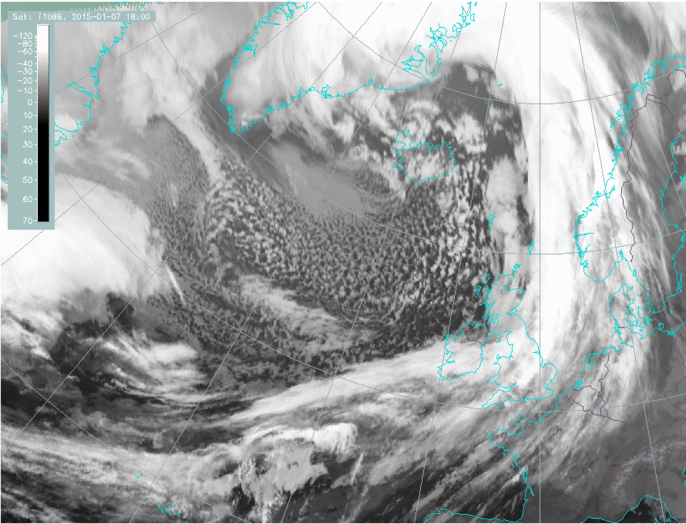
Fig. 10: 9 7 January 2015, 18 UTC - 9 January 2015, 06 UTC, 15 minute image loop; IR 10.8.

Meteorological And Physical Background

A Rapid Cyclogenesis is accompanied by distinct and typical cloud configurations in satellite images. Other names have been used in the literature to describe the same conceptual model, such as "explosive cyclogenesis" or "bomb" as well as names which describe only parts of the whole conceptual model, such as "emerging cloud head", "cyclogenesis within the left exit region of a jet streak" or "comma cloud".

1. Polar front theory and Rapid Cyclogenesis

The biggest differences between the the developments of classical polar fronts and Rapid Cyclogenesis are in the first phase. Here that is taken to be the stage between the first sign of a V-pattern (dry slot) and the development of a cloud spiral.

While a classical cyclogenesis through wave development is often slow and the wave bulge dissolves after some time or produces a spiral only after some days, the development of a Rapid Cyclogenesis is faster. The dry slot (V-pattern) typically evolves into a cloud spiral within 12 hours. After the mature stage is reached there is no longer any notable difference between the two processes.

The fast development of Rapid Cyclogenesis in its initial stage cannot be explained within the framework of the classical polar front theory developed by Bjerknes and Solberg (see Meteorological Physical Background of "Occlusion warm conveyor belt" and "Occlusion cold conveyor belt"). Consequently we must consider other processes and conditions that lead to rapid and intensive development.

From the features of WV and Airmass RGB images it is evident that sinking dry air has a significant impact on the cloud configuration.

2. Conveyor Belt Model

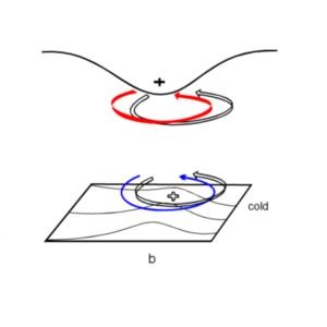
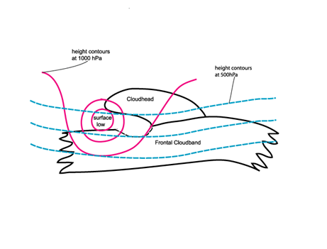
Features like a protruding cloud head suggest the theory of relative streams (see Basics, relative streams) as a likely method of investigation for a deeper understanding of cloud configurations.

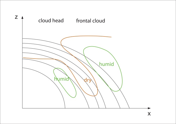
As shown in the conceptual models "Occlusion: Cold Conveyor Belt Type" and "Occlusion: Warm Conveyor Belt Type" there are several conveyor belts involved in the development of a cyclogenesis, resulting in different cloud systems. This can be seen in the schematics below. The cloudiness of the main frontal zone is produced by a typical warm conveyor belt together with a humid relative stream from behind, the "upper relative stream" while the dry stream from behind, the dry intrusion, appears behind the poleward edge of the frontal cloud band. This stream often contains stratospheric air.

As the schematics of the initial stages show, the warm conveyor belt and dry intrusion are also involved in the rapid cyclogenesis types. But there are also differences to the classical occlusion types: the cloud head of a Rapid Cyclogenesis is formed within the lower and mid-levels of the troposphere by a rapidly ascending relative stream (conveyor belt) from the south, which advects moist air from lower latitudes beneath the warm conveyor belt of the frontal zone. This relative stream of a Rapid Cyclogenesis has several similarities with the cold conveyor belt in the polar front theory of cyclogenesis, which also is an ascending relative stream below the warm conveyor belt, forming the cloudiness of the occlusion spiral. But such a cold conveyor belt usually originates from the east and is usually less warm and humid. So, it is not evident if the cold conveyor belt in connection with an occlusion spiral and the ascending relative stream in connection with the cloud head are same or comparable.

After crossing the cold front zone the ascending conveyor belt often splits into two branches that flow east and west. This splitting of the relative flow leads to the convex-shaped cloud edge at the poleward side of the cloud head. Also a cold conveyor belt sometimes shows this splitting effect.

As the advected air of the dry intrusion originates from the upper troposphere and the lower stratosphere, this flow is characterized by high values of potential vorticity. A potentially unstable stratification of the troposphere develops in the area where the dry intrusion flow over the ascending conveyor belt from the south. This is one of the factors that contribute to the development of convective storms in the same area (see the chapters 'Weather events' and 'Cloud structure in satellite images'). This is indicated in the schematic of the Advanced Stage below.

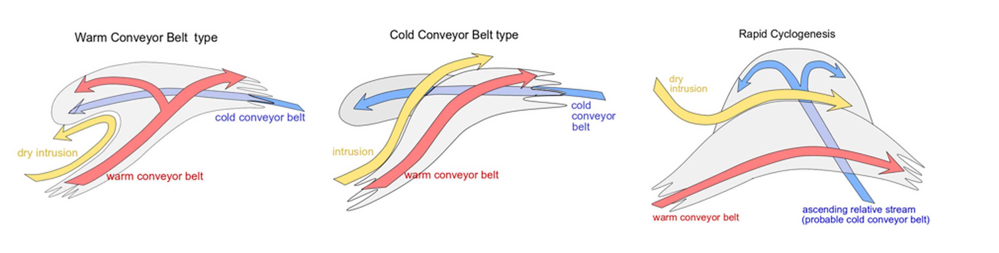
Fig. 11a: Development stages

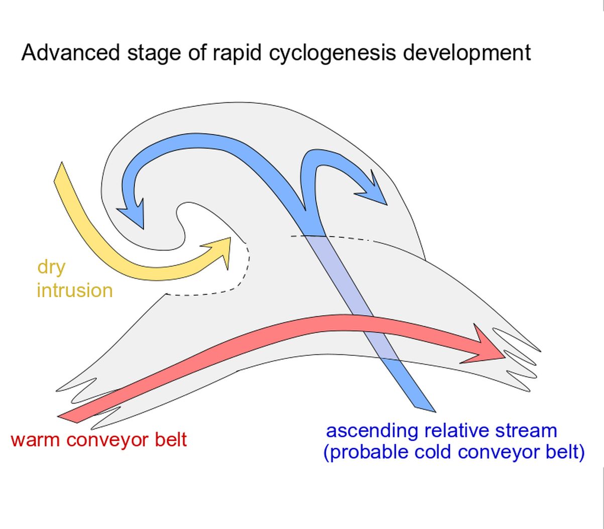
Fig. 11b: Advanced stage

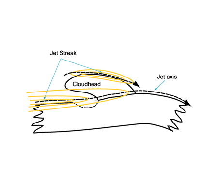
3. Jet, Jet streaks and 4-Quadrant Model by Uccellini

As mentioned above, the speed of a rapid cyclogenesis's development cannot be explained with the polar front theory alone; a different process is needed for a more detailed explanation. Rapid developments take place in the left exit region of jets and jet streaks. The structure of dark stripes along the rear edge of the frontal cloud band, which is best seen in WV images and Airmass RGB, also indicate that jets play an important role in the process of a Rapid Cyclogenesis.

Therefore, in addition to the development models of polar fronts and conveyor belts, upper air phenomena like the 4-quadrant jet streak model from Uccellini are taken into consideration and - as will be shown - play key roles.

Jet streaks can have straight or curved axes; during the initial stages of a Rapid Cyclogenesis the axes are mostly straight.

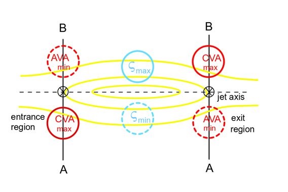
Fig. 12: Jet streak model

Jet streaks are the areas of maximum wind speed within the jet streams. The most interesting regions from the viewpoint of cyclonic developments are the entrance region where air particles accelerate, and the exit region where the air particles decelerate. As a consequence of these accelerations ageostrophic wind components develop in these regions, which leads to vertical movements.

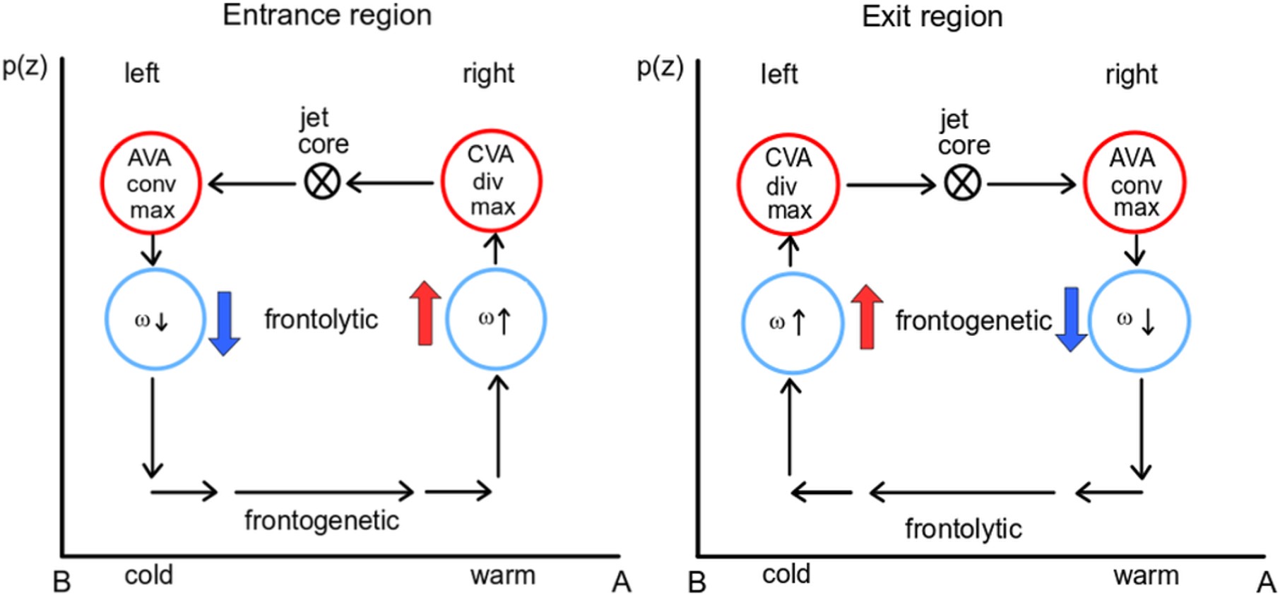
Fig. 13: Vertical cross section of a jet

Both entrance and exit regions are favorable for frontogenesis, although in different ways.

In the entrance region the frontogenetic process occurs mostly in the lower troposphere, which causes the process to last a longer time, typically more than 24 hours.

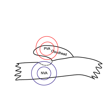
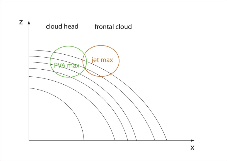
In the exit region the frontogenetic area lies in the middle troposphere, where the PVA maximum connects to the left exit region. These circumstances favour a rapid (under 12 hours) cyclogenesis.

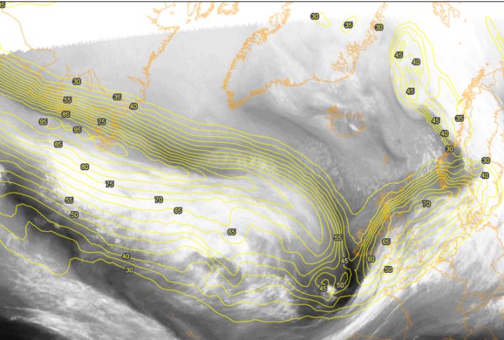
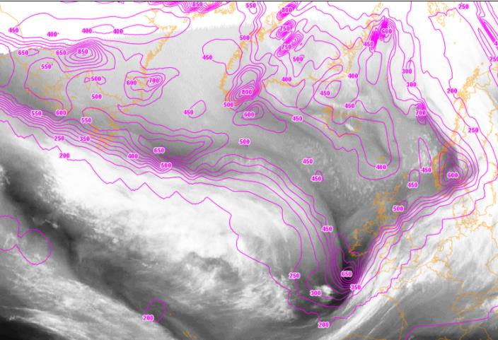
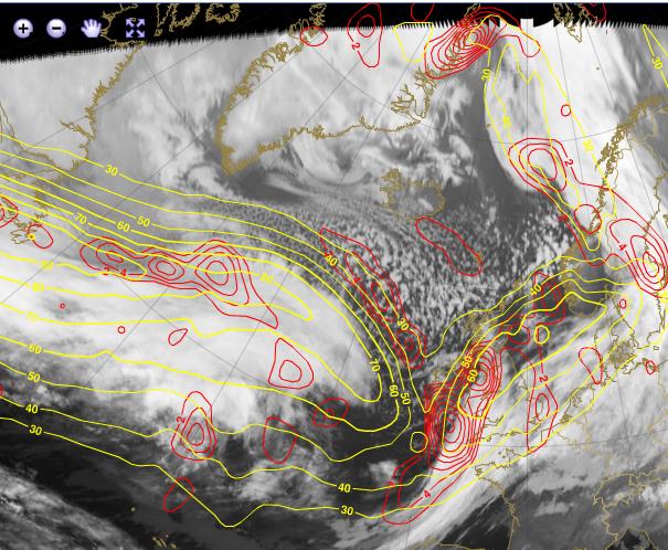
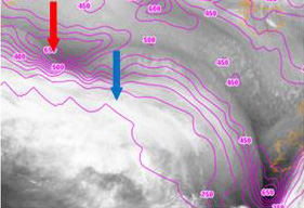
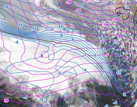
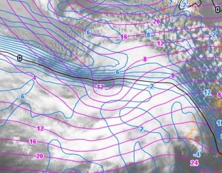
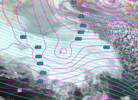
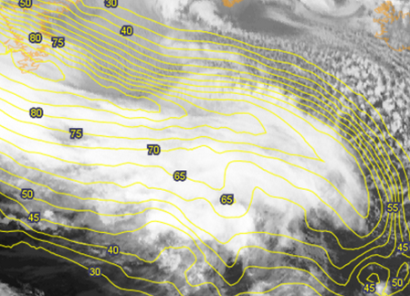
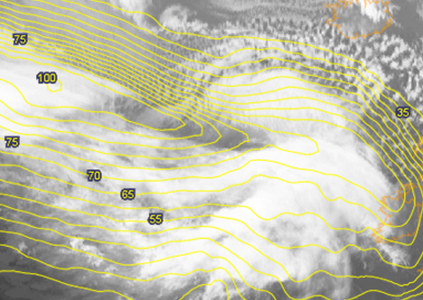
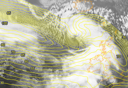
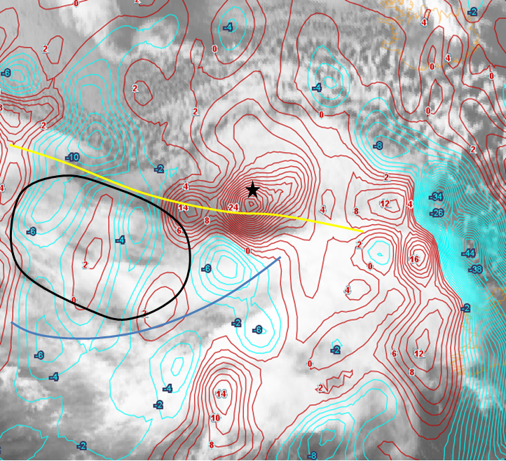
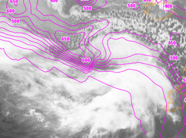
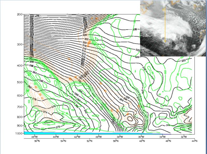
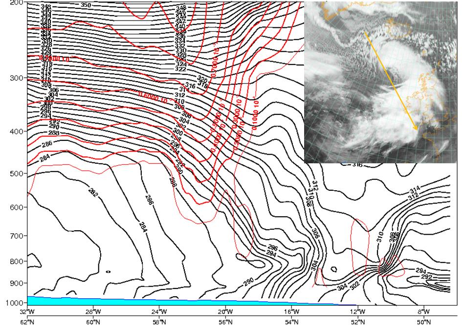
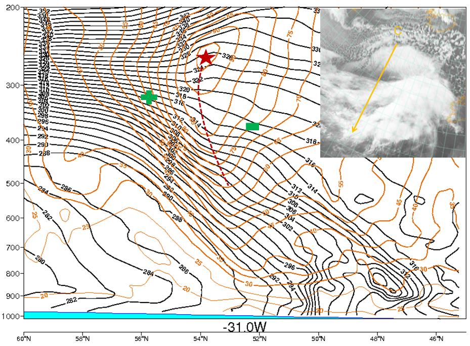
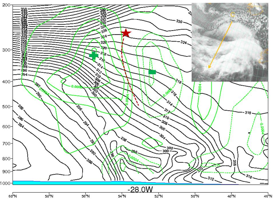
The jet stream axis lies parallel to the frontal cloud band with dry stratospheric air approaching the cloud head. This is the black stripe typically seen in WV imagery. Also, the PV values there are higher than 1 PVU. The emerging cloud head in the initial and development stage of the Rapid Cyclogenesis usually appears in the left exit region of a jet streak. This can be seen in the following WV 6.3 μm image from 8 January 2015 at 06 UTC with isotachs at 300 hPa, height of PVU > 2 and the PVA maximum at 300 hPa superimposed.

Fig. 14a: 8 January 2015, 06:00 UTC - Meteosat 10, WV 6.2 image. Yellow: isotachs 300 hPa.	Fig. 14b: 8 January 2015, 06:00 UTC - Meteosat 10, WV 6.2 imege. Magenta: height of PV >= 1 PVU.
Fig. 14c: 8 January 2015, 06:00 UTC - Meteosat 10, IR 10.8 image. Yellow: isotachs 300 hPa; red: positive vorticity advection 300 hPa.

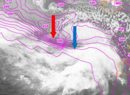
While there is ascending motion below the left exit region of the jet streak, descent takes place below the right exit region.

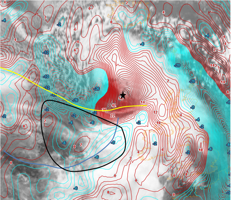
Quite often, and especially in cases with Rapid Cyclogenesis, this sinking motion leads to the dissolution of the cold front cloudiness. This can be seen clearly in the following image from 8 January 2015. The green star indicates the right exit region of the jet streak, where the cold front cloudiness has dissolved.

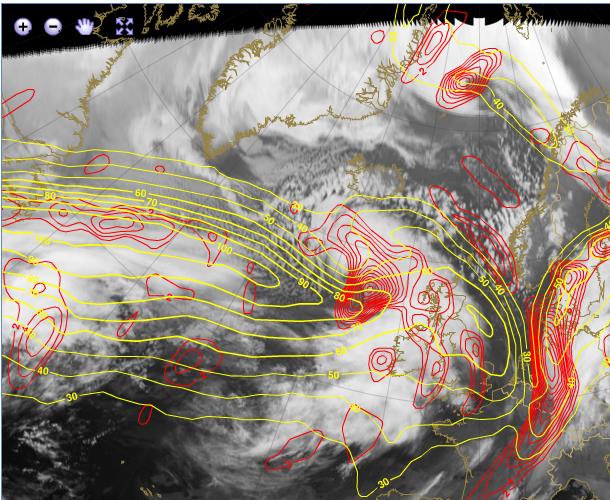
Fig. 15: 8 January 2015, 18 UTC - Meteosat 10; IR 10.8 image; yellow: isotachs 300 hPa; red: positive vorticity advection 300 hPa.

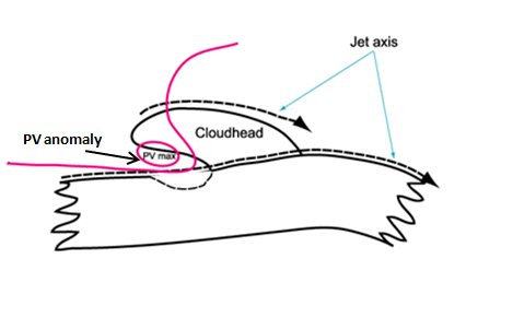
In summary, the part of the cloud head where the rapid development happens is an area of upward motion and cyclogenesis in the left exit region of a jet streak, and at same time an area where stratospheric air has protruded far downward, a so-called PV anomaly. This last fact in particular shows a difference between a classical polar frontal cyclogenesis and a Rapid Cyclogenesis; while in the case of classical wave development stratospheric air (if present at all) reaches the layer between 300 and 500 hPa, in the case of Rapid Cyclogenesis stratospheric air is a key feature and protrudes much further downward, with 500 hPa reached in the beginning of the process. This development process in the left exit region goes hand in hand with the dissolution of cold front cloudiness in the right entrance region.

4. Potential Vorticity

As demonstrated before, the development conditions in the left exit region of a jet streak can explain the rapid developments. On the other hand, there are also cases - especially in the cold conveyor belt (CCB) occlusion conceptual model - where the occlusion cloud band lies in the left exit region and thus under its physical influence. Therefore, there must still be yet another process to explain why some polar front developments are rapid and some are not.

The development of Rapid Cyclogenesis can be explained by the theory described by Hoskins et al. involving potential vorticity anomalies and their interaction with low-level baroclinic zones. (Compare: Basics/Numerical Parameters for Synoptic- to Mesoscale Cloud Systems /Potential Vorticity)

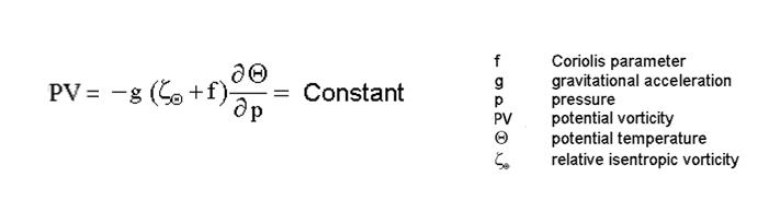
Fig. 16: Potential vorticity equation

When stratospheric air protrudes downward into the troposphere an upper level PV anomaly develops. As a consequence of the PV equation, positive vorticity will become more cyclonic because of the influence of the less stable environment of the troposphere.

When a positive upper level PV anomaly is being advected over a zone of strong, low-level temperature gradient a rotation is induced in the lower levels of the baroclinic zone, which causes warm advection at these levels and intensifies the cyclonic vortex there.

What takes place is a mutual intensification of cyclonic rotation from high to low and from low to high levels. The downward protrusion of high PV values can be seen in vertical cross sections. This does not mean that stratospheric air reaches the surface layers, but that the protrusion intensifies rotation in the lower layers.

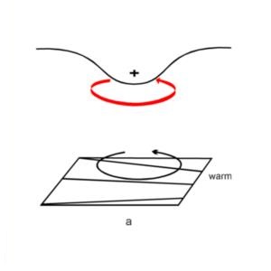
In the schematic below the thick solid arrow around the PV maximum indicates the cyclonic rotation. This rotation is induced at lower levels of the baroclinic zone as shown by the thin solid circulation arrow. This low level circulation causes warm advection ahead leading to a low level positive temperature anomaly indicated by the open + sign in the right figure (b). This temperature anomaly is associated with a cyclonic vortex which is marked by the open arrow at low levels. In turn, this circulation has a positive feedback to the upper troposphere, shown by an open circulation arrow at higher levels.

Fig. 17a: Positive PV anomaly.	Fig. 17b: Positive PV anomaly causing positive temperature advection.

At the same time another process is taking place: The induced low level vortex results in a strong equatorward wind component under the upper level PV anomaly. This southward component also influences the higher levels and leads to an equatorward advection of the upper level PV-anomaly which in turn intensifies the upper level wave.

Within this increased flow higher PV values to the west of the PV-anomaly are advected southward and lower PV values to the east of the PV-anomaly are advected northward. As a consequence of the latter process, the eastward movement of the PV-anomaly is decreased. Hence, the interaction between low and upper level circulations and the already ongoing cyclogenesis process will strengthen.

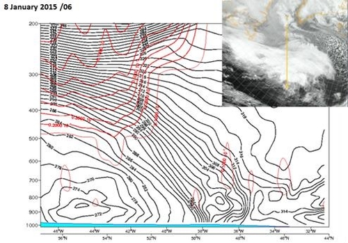
The next three images show the development of a Rapid Cyclogenesis. A PV anomaly (red arrow) protrudes downward and approaches the location of the surface low center (blue arrow) and simultaneously the cloud head turns into a cloud spiral.

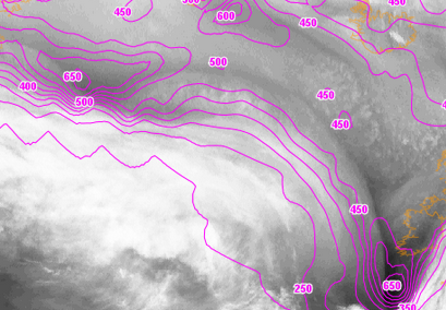
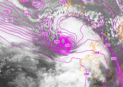
At 06 UTC an intensive PV anomaly is located behind the cloud head, parallel to the frontal cloud band. The (dynamical) tropopause, here indicated with the height of 1 PVU, has lowered to a minimum level of 650 hPa. Six hours later a V pattern has developed. At 18 UTC the PV anomaly has reached the location of the surface low and lowered to 950 hPa.

Fig. 18a: 8 January 2015, 06:00 UTC - Meteosat 10; WV 6.2 image. Magenta: height of PV>2 PVU; red arrow: PV>2PVU height maximum; blue arrow: low at 1000 hPa.	Fig. 18b: 8 January 2015, 12:00 UTC - Meteosat 10; WV 6.2 image. Magenta: height of PV>2 PVU; red arrow: PV>2PVU height maximum; blue arrow: low at 1000 hPa.
Fig. 18c: 8 January 2015, 18:00 UTC - Meteosat 10; WV 6.2 image. Magenta: height of PV>2 PVU; red arrow: PV>2PVU height maximum; blue arrow: low at 1000 hPa.

In the following vertical cross sections the downward protrusion of the PV anomaly is seen even more clearly: the minimum of 950 hPa was already reached by 12 UTC.

Fig. 19a: 8 January 2015, 06:00 UTC - vertical cross section. Black: isentrops; red: potential vorticity (PV); heavy > 2 PVU (stratospheric values); light: < 2 PV units (tropopsheric values).	Fig. 19b: 8 January 2015, 12:00 UTC - vertical cross section. Black: isentrops; red: potential vorticity (PV); heavy > 2 PVU (stratospheric values); light: < 2 PV units (tropopsheric values).
Fig. 19c: 8 January 2015, 18:00 UTC - vertical cross section. Black: isentrops; red: potential vorticity (PV); heavy > 2 PVU (stratospheric values); light: < 2 PV units (tropopsheric values)

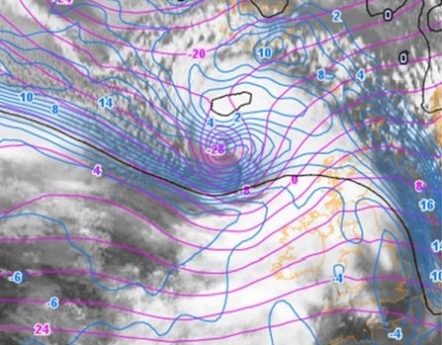
Another sign of the interaction between high and low layers is the movement and intensification of the surface low. In the beginning it is rather weak and situated on the anticyclonic side of the jet streak. During the development it moves to the cyclonic side and intensifies strongly when it encounters the left exit region. In the case of 8 January 2015 the height of 1000 hPa surface drops by 8 to 28 dam within 12 hours.

Fig. 20a: 8 January 2015, 06 UTC - Meteosat 10, IR 10.8 image. Magenta: height contours 1000 hPa; black/blue: shear vorticity 300 hPa; black: jet axis.	Fig. 20b: 8 January 2015, 12 UTC - Meteosat 10, IR 10.8 image. Magenta: height contours 1000 hPa; black/blue: shear vorticity 300 hPa; black: jet axis.
Fig. 20c: IR 10.8 image. Magenta: height contours 1000 hPa; black/blue: shear vorticity 300 hPa black: jet axis

5. Under discussion: Another Rapid Cyclogenesis development model

Another theory of cyclogenesis that also deviates from classical polar front theory has been discussed in the literature more and more often in the last decades. It is the Shapiro-Keyser cyclone model and it is mentioned here because some authors suggest that a Rapid Cyclogenesis is the result of this cyclogenetic process.

Although most of the presented case studies do not contain and take into account satellite images and the typical cloud configurations, the theory will be briefly summarized here.

According to the Shapiro-Keyser model, cyclogenesis deviates from Bjerknes and Solberg's polar front theory from a phase immediately after the wave development to the end stage of the spiral structure. The cold front is weak and soon dissipates from the warm front. In contrast, the warm front is very strong and starts to rotate around the low center, creating a warm seclusion. This development often occurs in west-east oriented fronts with air masses from warmer latitudes, and in the area of confluent flows in jet streak entrance regions.

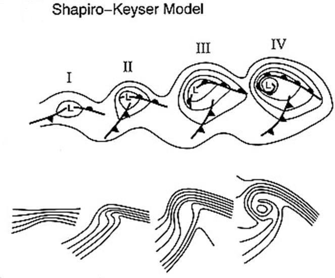
Fig. 21: Shapiro-Keyser cyclogenesis model

The polar front theory of Bjerknes and Solberg is an occlusion process in which a cold front catches up to a warm front and lifts warm air upward. The Shapiro-Keyser model is based on the idea of wrapping the different air masses around the center, resulting in the warm seclusion.

There are some similarities between Rapid Cyclogenesis events and the Shapiro-Keyser model, such as the west-east orientation of the frontal system, the very intensive warm advection in the warm front and cloud head cloudiness (especially in the beginning of the process), the dissolution of cold front cloudiness in a more advanced stage, and, in nearly all cases, a recognizable cloud spiral around the low center in the final stage.

However, Rapid Cyclogenesis also deviates from the Shapiro-Keyser model in important ways. In the case of Rapid Cyclogenesis, the main development takes place in the left exit region of a jet streak, which is to say: in the diffluence and not the confluence area of a jet streak. Also, if one looks into the development of cloud configurations in satellite images, frontal (especially warm front) cloudiness and cloud heads are clearly different configurations which are best explained with conveyor belts.

Further investigation is recommended to clarify the open questions.

Key Parameters

• Height contours at 1000 hPa and 500 hPa:

The height contours at 1000 hPa start with a weak low or trough but undergo rapid deepening during the initial stages of development. The upper level height contours at 500 or 300 hPa show only a very weak trough in the beginning to the west of the surface low. The trough deepens during the process and finally catches up with the position of the surface low. The height contours at 500 (or 300) hPa are perpendicular to the height contours at 1000 hPa in the initial phases, indicating the cyclogenesis is in the developing stage.

The mature stage is characterized by a low center with very low values at 1000 hPa as well as at 500/300 hPa. At this point the trough axis is vertical and situated in the center of the cloud spiral.

• Temperature advection (TA):

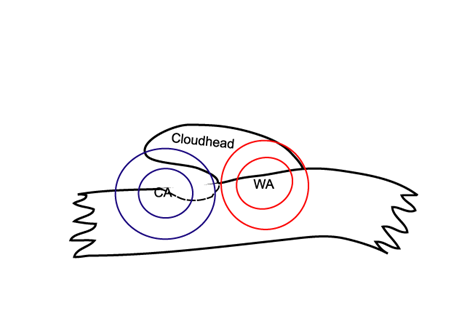
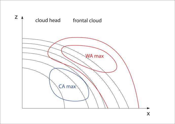
The field of temperature advection shows a very typical situation for a wave: a maximum of warm advection (WA) within the cloud head and the warm front (WF) shield and cold advection (CA) behind. This pronounced WA/CA dipole is a sign of the ongoing cyclogenesis. However, one characteristic of Rapid Cyclogenesis events is that compared to more classical developments the WA is very strong, with values sometimes even higher than those of the CA.

• Isotachs at 300 hPa:

The isotachs at 300 hPa show a pronounced jet streak along the rear edge of the frontal cloud band. The cloud head can be found within the left exit region of this jet streak. In the mature stage a second jet streak often forms at the east-northeastern (polar) side of the cloud head.

• Vorticity advection at 500 and 300 hPa (positive vorticity advection or PVA, and negative vorticity advection or NVA):

The field of vorticity advection shows a pronounced PVA maximum at 500 and 300 hPa, situated mostly within the area of the cloud head and therefore also in the area of the left exit of the main jet streak. If the second jet streak, downstream from the low, has already developed, the maximum is also located near the right entrance of the second jet streak. As a consequence both PVA maxima work together and have an enhanced impact.

During the phase of strongest development NVA in the right exit region intensifies, which goes hand in hand with the dissipation of clouds within the cold front of the cold front cloud band.

• Potential vorticity (PV):

The potential vorticity shows a PV anomaly (values bigger than 1 PVU) protrude downward in the upper troposphere along the rear cloud edge of the cold front.

The anomaly, which separates tropospheric and stratospheric air, goes lower than in classical cyclogenesis. In the initial stage it is approximately at 400-500 hPa and goes down to 700 hPa or even lower. In the beginning of the process the anomaly is upstream of the low center, and approaches it while the Rapid Cyclogenesis proceeds.

In the phase where the deepening of the surface low is strongest, the PV anomaly coincides with the location of the low and the intensified PV values of the troposphere.

This does not automatically mean that stratospheric air reaches the surface. The increase of PV in the low layers can also have other reasons, such as the mutual increase of rotation between high and low levels as described by Hoskins (see Meteorological Physical Background) and the release of latent heat, especially in convective situations.

The images from 8 January 2015 show three time steps in the life cycle of a Rapid Cyclogenesis: 06:00, 12:00 and 18:00 UTC from initial to advanced stage. The schematics summarize the most typical features which can appear in some or all phases of development.

Height contours at 1000 hPa and 500 (300 hPa)

Fig. 22a: Schematic of height contours at 1000 hPa and 500 hPa.	Fig. 22b: 8 January 2015, 06:00 UTC - Meteosat 10, IR 10.8 image. Magenta: height contours 1000 hPa, cyan: height contours 500 hPa.
Fig. 22c: 8 January 2015, 12:00 UTC - Meteosat 10, IR 10.8 image. Magenta: height contours 1000 hPa, cyan: height contours 500 hPa.	Fig. 22d: 8 January 2015, 18:00 UTC - Meteosat 10, IR 10.8 image. Magenta: height contours 1000 hPa, cyan: height contours 500 hPa.

Temperature advection (TA) at 700 hPa

Fig. 23a: Schematics of temperature advection.	Fig. 23a: 8 January 2015, 06:00 UTC - Meteosat 10, IR 10.8 image. Temperature advection 700 hPa; red: warm advection; blue: cold advection.
Fig. 23b: 8 January 2015, 12:00 UTC - Meteosat 10, IR 10.8 image. Temperature advection 700 hPa; red: warm advection; blue: cold advection.	Fig. 23c: 8 January 2015, 18:00 UTC - Meteosat 10, IR 10.8 image. Temperature advection 700 hPa; red: warm advection; blue: cold advection.

Isotachs at 300 hPa

Fig. 24a: Schematics of isotachs at 300 hPa.	Fig. 24b: 8 January 2015, 06:00 UTC - Meteosat 10, IR 10.8 image. Yellow: isotachs 300 hPa.
Fig. 24c: 8 January 2015, 12:00 UTC - Meteosat 10, IR 10.8 image. Yellow: isotachs 300 hPa.	Fig. 24d: 8 January 2015, 18:00 UTC - Meteosat 10, IR 10.8 image. Yellow: isotachs 300 hPa.

Vorticity advection at 300 hPa (PVA/NVA)

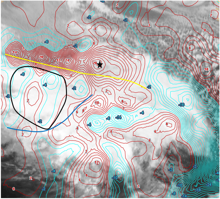
The field of vorticity advection is rather noisy and it is important to filter out the meteorologically irrelevant areas from the important ones. To make this easier the relevant PVA fields are marked by a black star and the NVA areas are encircled by a black line.

Fig. 25a: Schematics of vorticity advection at 300 hPa.	Fig. 25b: 8 January 2015, 06:00 - Meteosat 10, IR 10.8. image. Vorticity advection 300 hPa; red: PVA; cyan: NVA; blue line: TFP CF; yellow line: jet axis 300 hPa; black line: CF cloud dissolution.
Fig. 25c: 8 January 2015, 12:00 - Meteosat 10, IR 10.8. image. Vorticity advection 300 hPa; red: PVA; cyan: NVA; blue line: TFP CF; yellow line: jet axis 300 hPa; black line: CF cloud dissolution.	Fig. 25d: 8 January 2015, 18:00 - Meteosat 10, IR 10.8 image. Vorticity advection 300 hPa; red: PVA cyan: NVA; blue line: TFP CF; yellow line: jet axis 300 hPa; black line: CF cloud dissolution.

Potential Vorticity (PV)

Fig. 26a: Schematics of potential vorticity	Fig. 26b: 8 January 2015, 06:00 UTC - Meteosat 10, IR 10.8 image. Magenta: height of PV >1 unit.
Fig. 26c: 8 January 2015, 12:00 UTC - Meteosat 10, IR 10.8 image. Magenta: height of PV >1 unit.	Fig. 26d: 8 January 2015, 18:00 UTC - Meteosat 10, IR 10.8 image. Magenta: height of PV >1 unit.

Typical Appearance in Vertical Cross Sections

• Moist isentropes

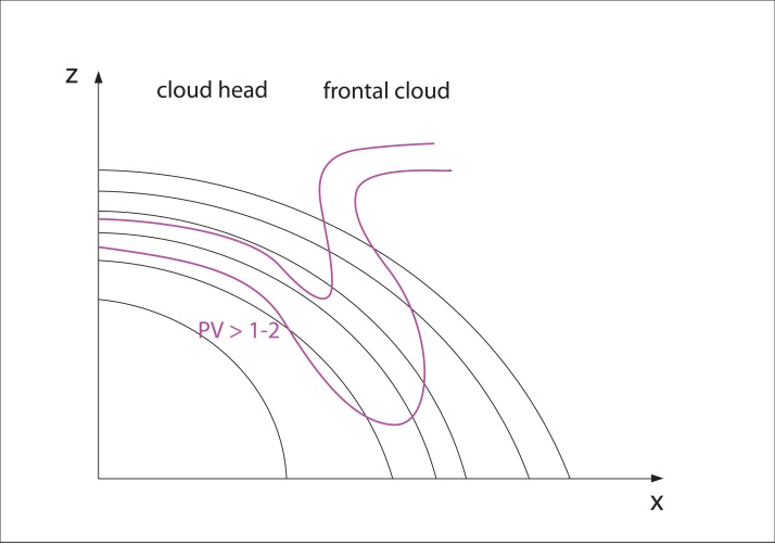
The isolines of moist isentropes form a downward-inclined zone with a high gradient typical for cold fronts. In the case of a Rapid Cyclogenesis the zone is broad and contains isolines of both the cold front and the cloud head, which are close to each other, or even merge together.

In the initial stages, where the cold front and cloud head are clearly separated, there is often a double structure within this zone as well. This double structure vanishes as the distinct cloud spiral develops.

• Relative humidity:

The relative humidity is high within the frontal cloud band and cloud head. In between them, within the dry tongue, can be found low values of relative humidity which reach from the tropopause down to relatively low levels in the atmosphere.

• Potential vorticity (PV):

Potential vorticity shows an anomaly protruding downward deep into the troposphere below the zone with the highest moist isentrope gradient in the cold front. This lowering of the so-called dynamical tropopause (1 - 2 PV Units) is already clearly seen in the initial stage, where the tropopause height sinks below about 400 hPa. In the mature stage the tropopause is usually below 500 hPa and in extreme cases below 700 hPa. At the same time there is an intensification of PV in the lowest tropospheric layer from the typical values of PV < 1 unit to PV > 1 unit and more. In the final phase a column of PV values > 1 unit develops and stretches from the stratosphere down almost to the surface.

• Temperature advection (TA):

The temperature advection shows a very distinct situation similar to but more pronounced than a classical wave; there is a maximum of warm advection within and ahead of the cloud head, and cold advection directly behind it.

• Vorticity advection (PVA/NVA):

The vorticity advection shows a pronounced PVA maximum in the upper levels, mostly situated within the cloud head, and an NVA maximum on the other side of the dry tongue in the gradient zone of the cold front. Both correlate well with the left and right exit regions of the jet streak.

• Isotachs:

The isotachs show a pronounced jet stream along the rear edge of the frontal gradient of the cold front. The cloud head can often be found within the left exit region of a jet streak situated upstream of the low. In later stages of development, another maximum of the isotachs is often present at the poleward side of the cloud head.

A sting jet can develop in the advanced development stage and mature stage. It can be seen as an isotach maximum below the frontal zone, reaching from the surface up to 700 hPa.

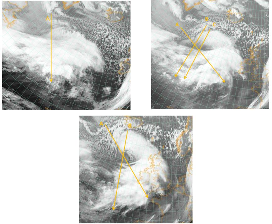
The images from 8 January 2015 show three time steps in the life cycle of a Rapid Cyclogenesis at 06, 12 and 18 UTC.

The cross sections are taken across the cloud head and the cold front from north-northwest to south-southwest through the deepening surface low and the developing dry intrusion. For the different stages of development slightly different cross sections were made to show the most indicative features of each stage.

Fig. 27a: 8 January 2015, 06:00 UTC - Meteosat 10, IR 10.8 image. Orange: location of vertical cross section A.	Fig. 27b: 8 January 2015, 12:00 UTC - Meteosat 10, IR 10.8 image. Orange: locations of vertical cross sections A, B and C.
Fig. 27c: 8 January 2015, 18:00 UTC - Meteosat 10, IR 10.8 image. Orange: locations of vertical cross sections A and B.

Relative Humidity

Fig. 28a: Schematics for moist isentropes and relative humidity: Initial and development stage.	Fig. 28b: 8 January 2015, 06:00 UTC - vertical cross section A. Black: moist isentropes (ThetaE), green/brown: relative humidity.

Potential Vorticity

Fig. 29a: Schematics for moist isentropes and potential vorticity (PV): all development stages.	Fig. 29b: 8 January 2015, 18:00 UTC - vertical cross section A. Black: moist isentropes (ThetaE), red: potential vorticity: heavy: > 2 PVU, light: < 2 PVU.

Temperature Advection

Fig. 30a: Schematics for moist isentropes and temperature advection: initial to advanced stages.	Fig. 30b: 8 January 2015, 12:00 UTC - vertical cross section A. Black: moist isentropes (ThetaE), temperature advection: red: warm advection; blue: cold advection.

Vorticity Advection and Isotachs

Fig. 31a: Schematics for moist isentropes, isotachs and vorticity advection: initial to advanced stages.
Fig. 31b: 8 January 2015, 12:00 UTC - vertical cross section A. Black: moist isentropes (ThetaE), brown: isotachs	Fig. 31c: 8 January 2015, 12:00 UTC - vertical cross section A. Black: moist isentropes (ThetaE), green: vorticity advection

Weather Events

Parameter	Description
Precipitation	Intense precipitation associated with the warm conveyor belt. Thunderstorms within the inner edge of the cloud head on the western side of the surface low. They can also develop within the dry slot.
Temperature	Substantial rise in surface temperature within the area of the warm conveyor belt.
Wind (incl. gusts)	Strong winds within the area of the cloud head. In extreme cases winds can reach hurricane force. Very strong gusts in the transition zone between dark and white as can be seen in the WV channels near the cold front and the cloud head. Possibility of the development of a sting jet in the advanced and mature stages in the southern semicircle of the low and south of the decaying cloud spiral. (see below) Sting jet cases may involve hurricane force winds with gusts up to 200 km/h.
Other relevant information	Very strong falls and rises in pressure. In the initial stage, falls ahead exceed the rises behind.

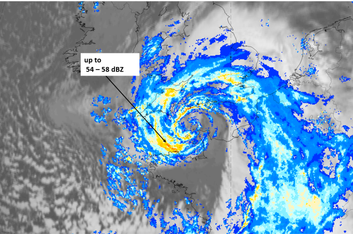
As just described, rapid cyclogenesis events are often connected with severe or even catastrophic weather events. As the development usually starts over the Atlantic, the severe weather is observed when it has already reached the “advanced” and “mature” development stages.

To show a few of the weather events, the case from 1-2 October 2020 is chosen.

Legend: 1-2 October 2020; IR images
Left: 1 October 18 UTC, development phase; central: 2 October 00 UTC, advanced phase; right: 2 October 06 UTC, mature phase.
*Note: click on the image to access the image gallery (navigate using arrows on keyboard)

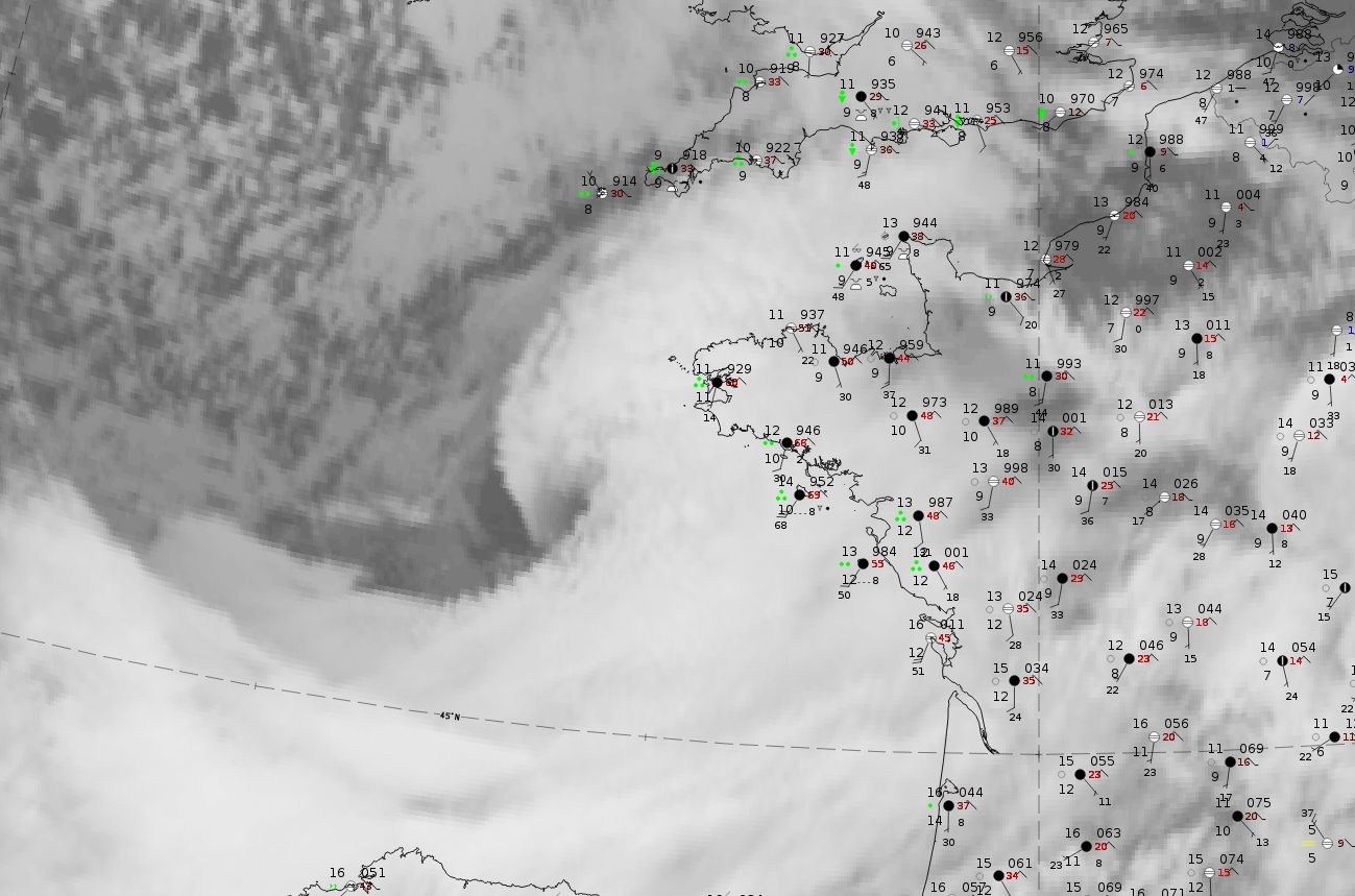
Development phase: 1 October 2020, 18 UTC

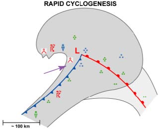
Fig. 32: Weather events at the ground level

Legend:
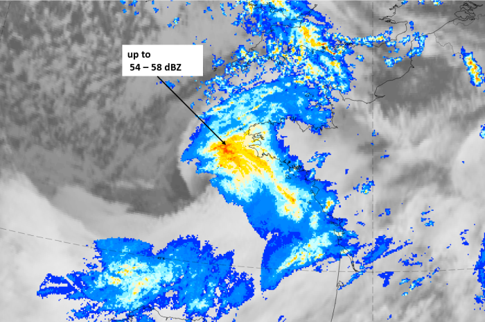
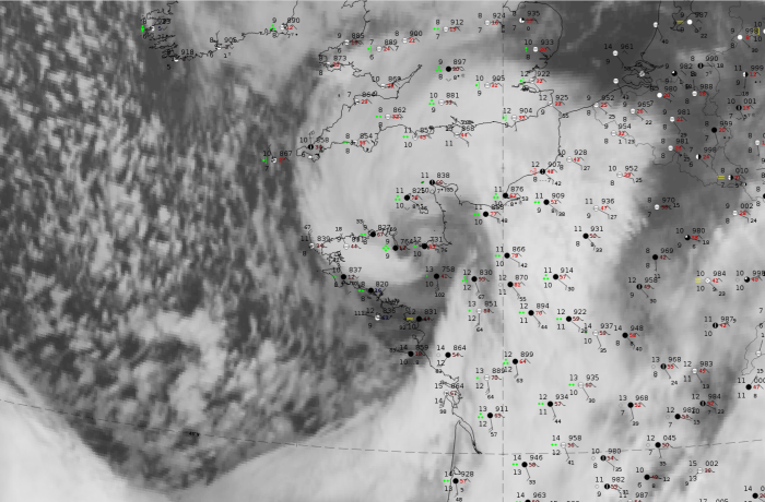
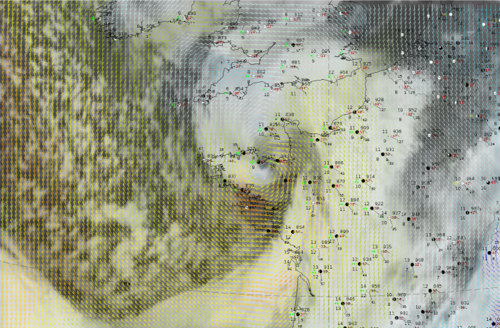
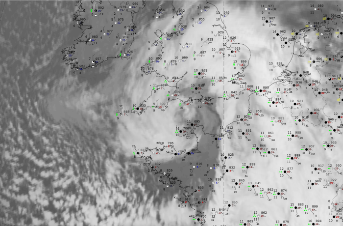
1 October 2020, 18UTC: IR + synoptic measurements (above) + probability of moderate rain (Precipitting clouds PC - NWCSAF).
Note: for a larger SYNOP image click this link.

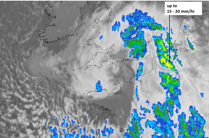
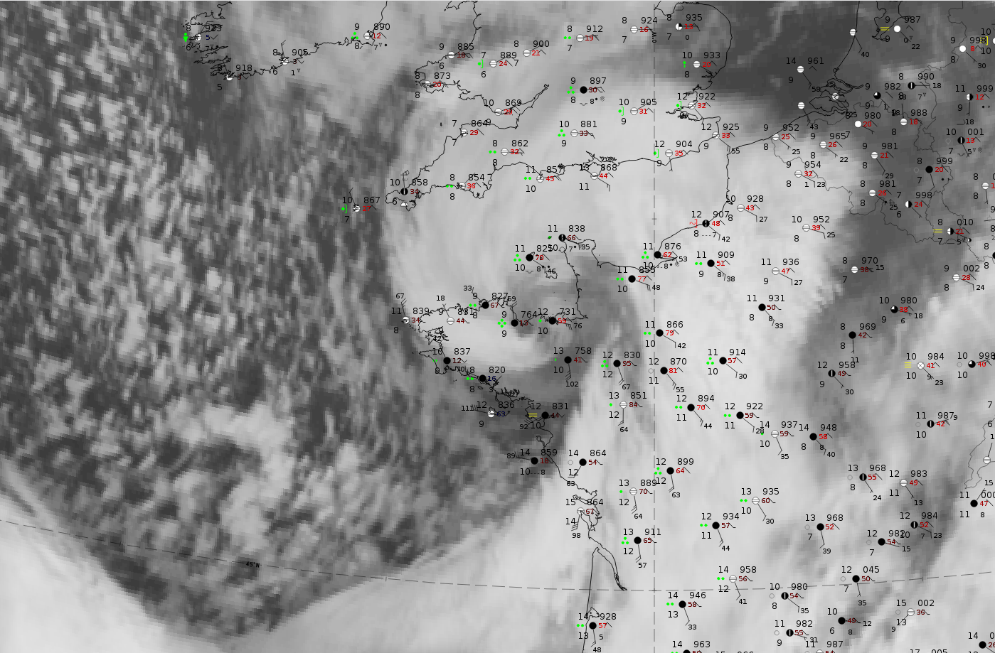
The development phase can be seen due to the visible dry slot southwest of Brittany and intensive precipitation events over the land to the east of the development area. The strongest surface winds appear to the south of the development area with speed values up to 55 knots.

Legend:
1 October 2020, 18 UTC, IR ; superimposed:
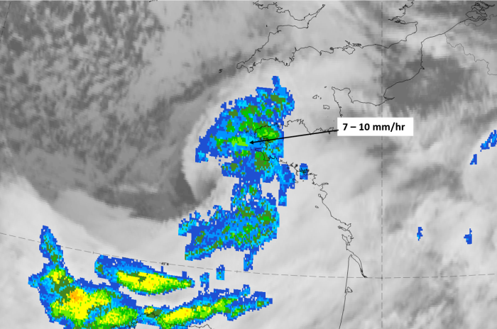
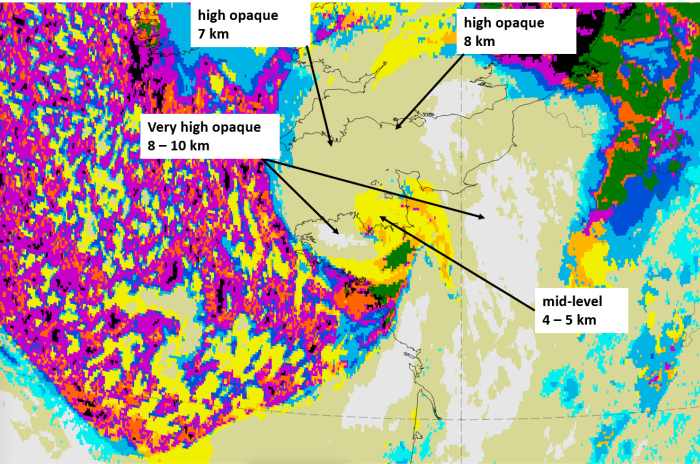
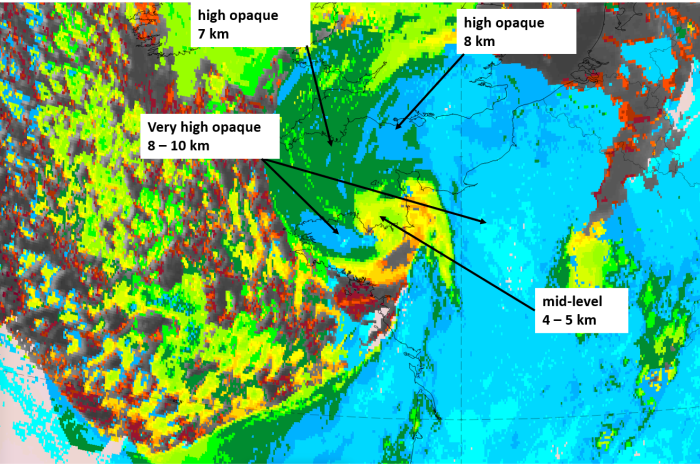
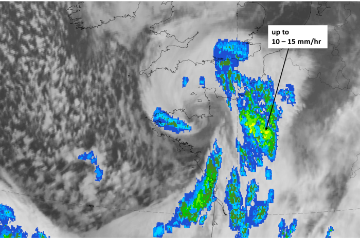
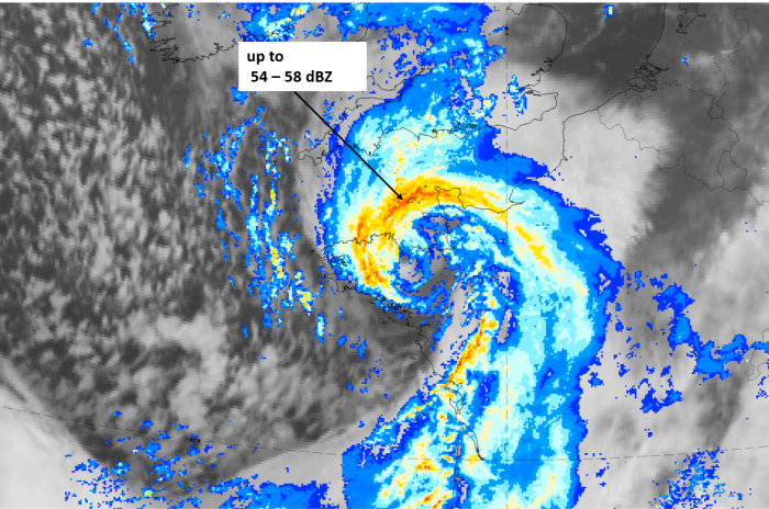
1st row: Cloud Type (CT NWCSAF) (above) + Cloud Top Height (CTTH - NWCSAF) (below); 2nd row: Convective Rainfall Rate (CRR NWCSAF) (above) + Radar intensities from Opera radar system (below).

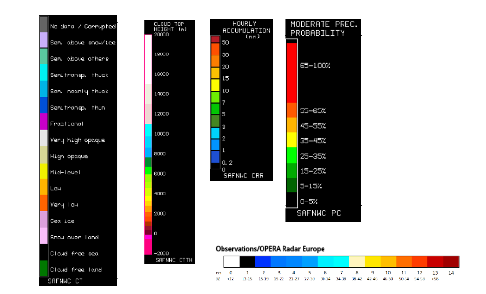
For identifying values for Cloud type (CT), Cloud type height (CTTH), precipitating clouds (PC), and Opera radar for any pixel in the images look into the legends. (link).

Advanced phase: 2 October 2020, 00 UTC

Fig. 33: Weather events at the ground level

Note: for a larger SYNOP image click this link.

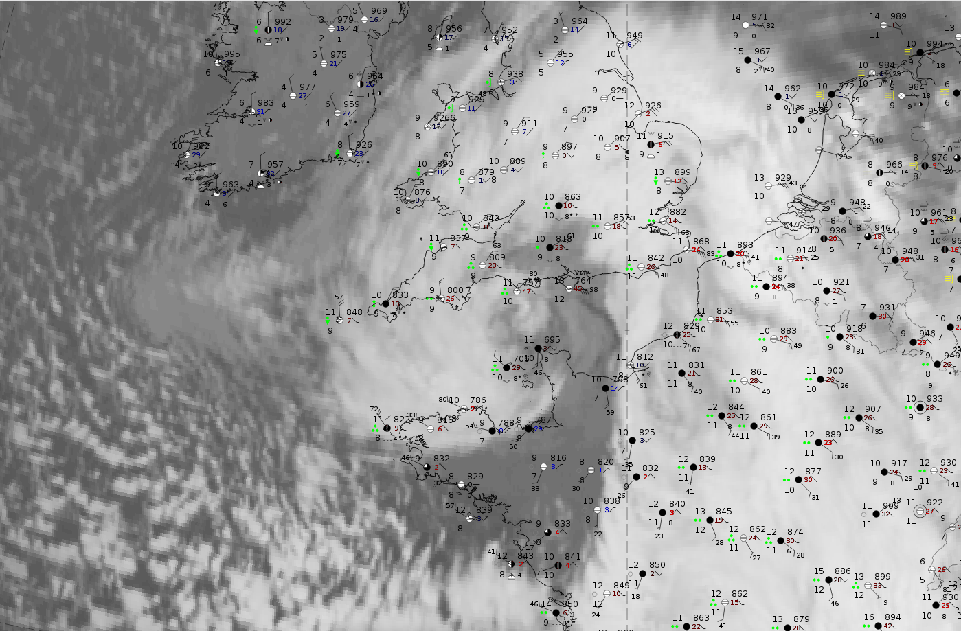
In the advanced stage which can be seen over Brittany and the Normandie there are wide-spread intensive precipitation events visible. The strongest surface winds appear immediately to the south of the spiral centre with speed values up to 50 knots.

2 October 2020, 00 UTC, IR; superimposed:
1st row: Cloud Type (CT NWCSAF) (above) + Cloud Top Height (CTTH - NWCSAF) (below); 2nd row: Convective Rainfall Rate (CRR NWCSAF) (above) + Radar intensities from Opera radar system (below).

For identifying values for Cloud type (CT), Cloud type height (CTTH), precipitating clouds (PC), and Opera radar for any pixel in the images look into the legends. (link).

Mature phase: 2 October 2020, 06 UTC

Fig. 34: Weather events at the ground level

Note: for a larger SYNOP image click this link.

In the mature stage, which is centred over the English Channel, there are still wide-spread intensive precipitation events. The strongest surface winds appear immediately to the north-east of the spiral centre with speed values up to 50 knots.

2 October 2020, 06 UTC, IR; superimposed:
1st row: Cloud Type (CT NWCSAF) (above) + Cloud Top Height (CTTH - NWCSAF) (below); 2nd row: Convective Rainfall Rate (CRR NWCSAF) (above) + Radar intensities from Opera radar system (below).

For identifying values for Cloud type (CT), Cloud type height (CTTH), precipitating clouds (PC), and Opera radar for any pixel in the images look into the legends. (link).

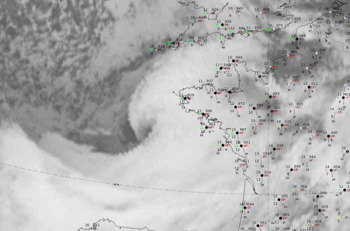
One important severe, even catastrophic, weather event taking place in the later development stages of a rapid cyclogenesis is the appearance of sting jets. For demonstrating such an event the case of 9 January 2015 is used, which also has banded cloud structures (discussed in the first chapter). The sting jet can be observed at 00 UTC.

Although the cloud spiral is not directly over land, heavy showers and high wind speed can be seen in synoptic measurements over the Hebrides (NW Scotland).

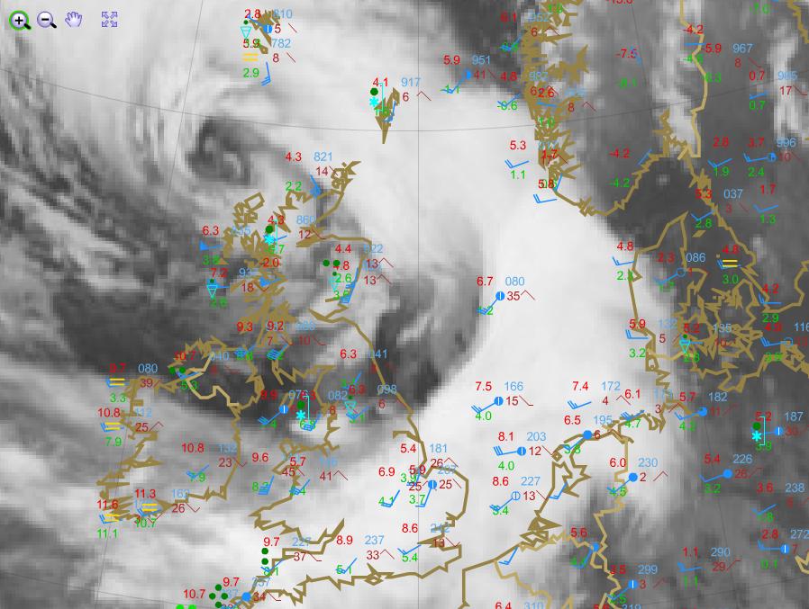
Legend: 9 January 2015, 00 UTC, Meteosat; IR 10.8 and synoptic observations.

Legend: 9 January 2015, 00 UTC, Meteosat; IR 10.8 and ECMWF 10m wind

The 10-meter wind speed maximum and its location, typical for a sting jet - discussed in the "Meteorological Physical Background" chapter - can be seen in the data from 9 January 2015, 00:00 UTC.

As already mentioned in the table above, sting jets may appear at the innermost part of the cloud spiral during the advanced and mature stages of a Rapid Cyclogenesis event.

A sting jet is a mesoscale (no wider than about 100 km) zone of fast moving air descending from a height of 3-4 km to the surface just south of the low centre. The high winds last only for a few hours, but they can cause widespread damage on the surface.

Sting jets may occur in connection with any intensive cyclogenesis. Their structure and development are not yet fully understood; both dynamical and thermodynamical approaches have been applied.

The next two images show the moist isentropes and isotachs in vertical cross sections (VCSs) from 8 January 2015 at 12:00 and 18:00 UTC. Both cross sections show the maximum of the upper level jet with the core between about 250 and 300 hPa. But during these 6 hours a second wind maximum has developed in the low layers with a core between 950 and 800 hPa.

Although it is not so easy to decide if this is a sting jet or some other wind speed maximum, these two figures do demonstrate the applicability of VCSs for a more detailed investigation of strong winds and the possibility of their damaging impact.

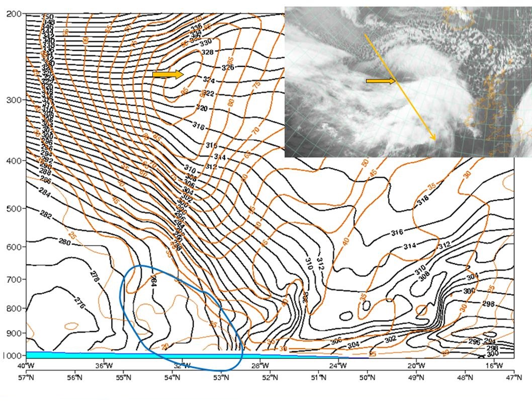
Fig. 35: 8 January 2015, 12:00 UTC - Meteosat 10, IR 10.8 image. Black: moist isentropes; brown: isotachs; yellow: orientation of VCS line; yellow arrow: position of upper level jet core; blue line: area under the front from the surface up to 700 hPa.

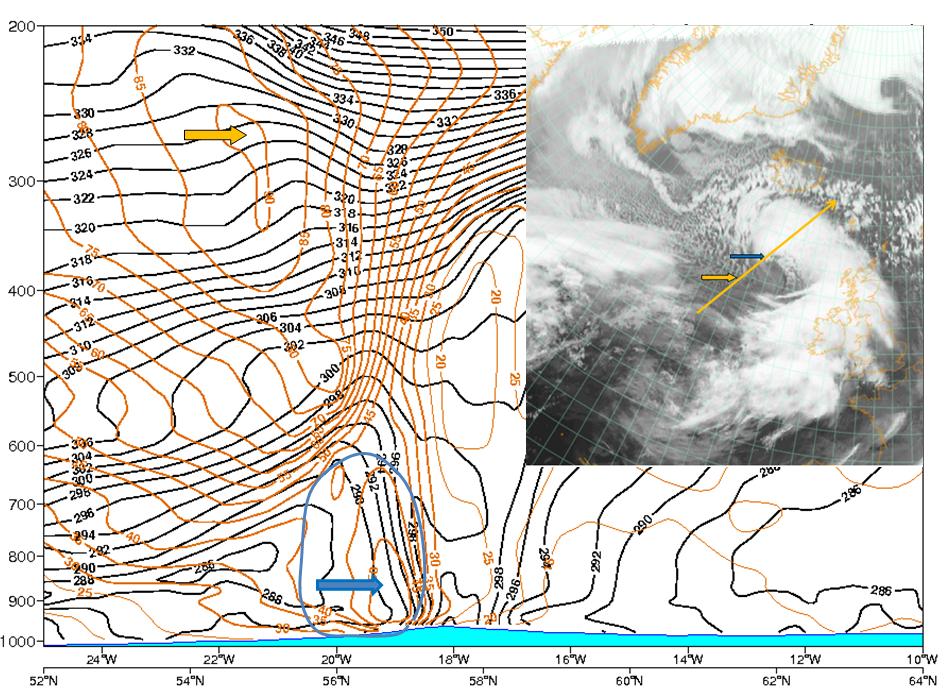
Fig. 36: 8 January 2015, 18:00 UTC - Meteosat 10, IR 10.8 image. Black: moist isentropes; brown: isotachs; yellow: orientation of VCS line; yellow arrow: position of upper level jet core; blue arrow: position of a low level jet (possibly a sting jet); blue line: area under the front from the surface up to 700 hPa.