Table of Contents
Cloud Structure In Satellite Images
In this study about 30 cases of Back Bent Occlusions from different time periods were investigated.
The most interesting information for a Back Bent Occlusion can be seen in the sequence of development stages. In the initial stage there is a quite straight or only slightly cyclonically curved occluded front. The occluded front stops moving, and after that the whole front or a part of it begins to move backwards. In most cases the occluded front is bent back by a cold advection originating from another low (usually an Upper Level Low; see Upper Level Low ) in a polar airmass.
Such a development can be seen in this 3-hourly sequence of IR-images from 6 January 2020 at 12 UTC to 7 January 2020 at 03 UTC.
Legend: 6 January 2020 at 12 to 7 January 2020 at 03 UTC; three-hourly; IR-images.*Note: click on the image to access the image gallery (navigate using arrows on keyboard)
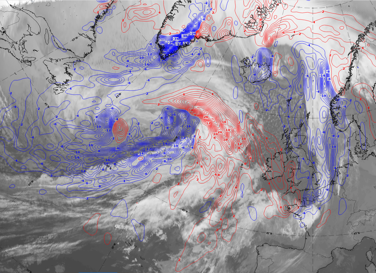
The low in upper levels north-east of the former occlusion cloud band and the connected cold air advection, on 6 January 2020 at 18 UTC, can be seen in the images below. Both are responsible for the change of an occlusion cloud band into a Back Bent Occlusion.
 |
Legend:
IR images from 6 January 2020 at 18 UTC; l: cyan: height contours 500 hPa; right: temperature advection at 700 hPa; red: warm advection, blue: cold advection.
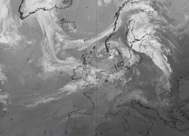
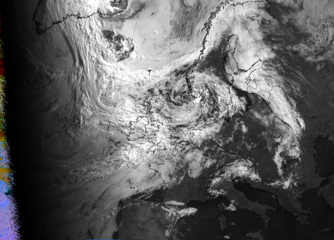
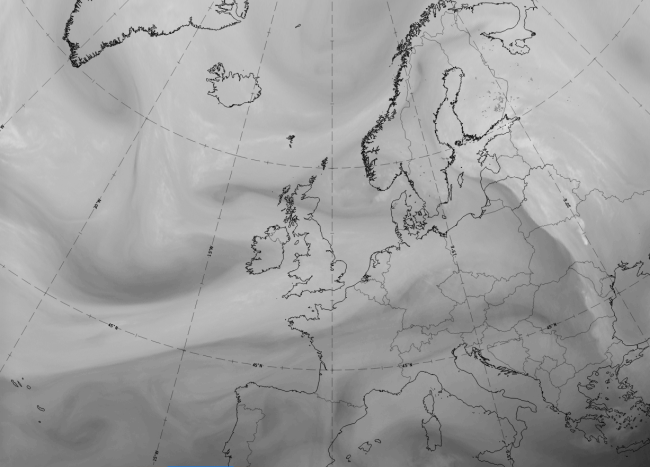
Appearance in the basic channels:
In most cases the cloud band related to the occluded front is long and broad, but there are also cases, especially in cold air masses, where the cloud band is short, narrow and somewhat inconspicuous in the satellite image
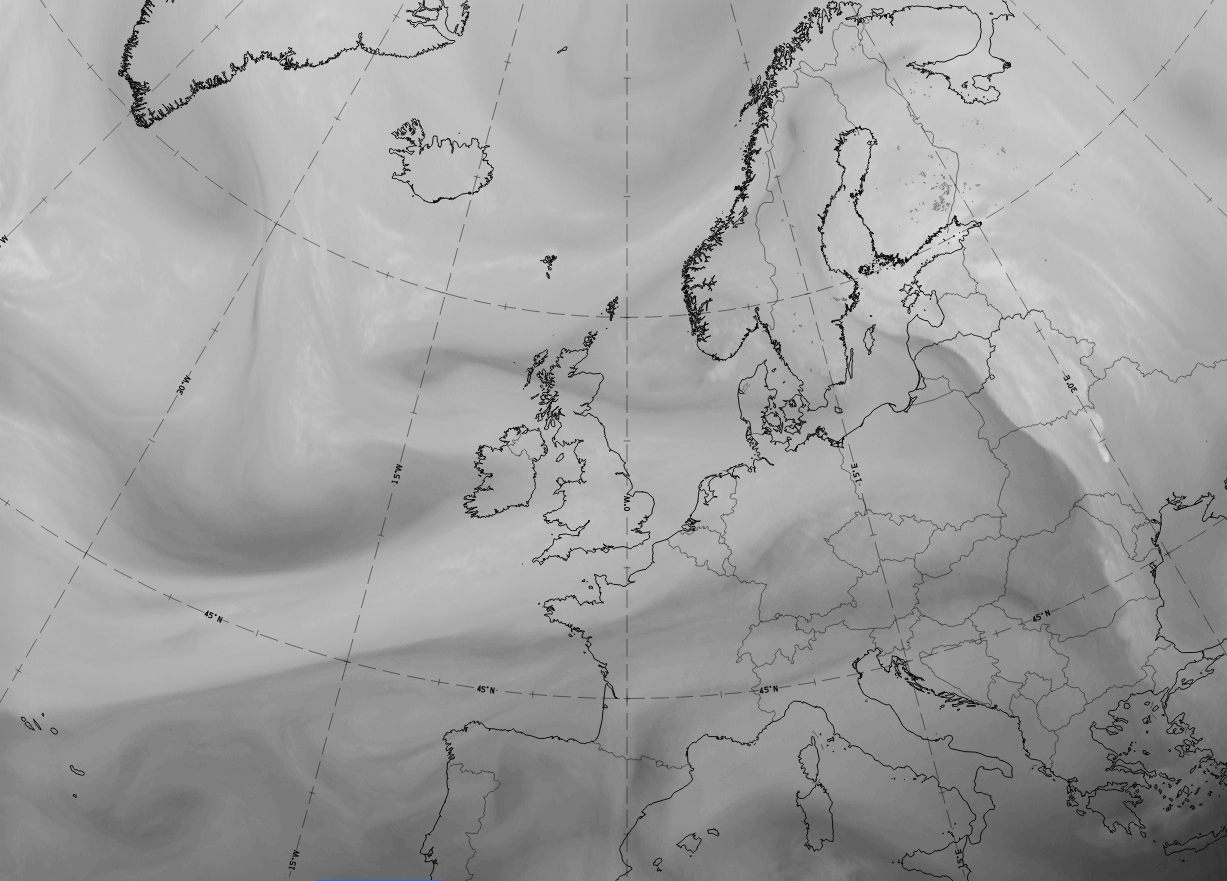
In most cases the IR and WV images of the cloud band related to the Back Bent Occlusion have grey colours, indicating rather lower cloud tops.
In the VIS images, white spots, lines and patches indicate thicker, higher-reaching clouds.
 |
 |
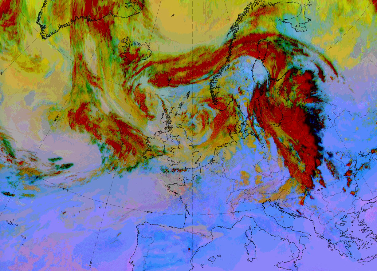
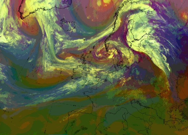
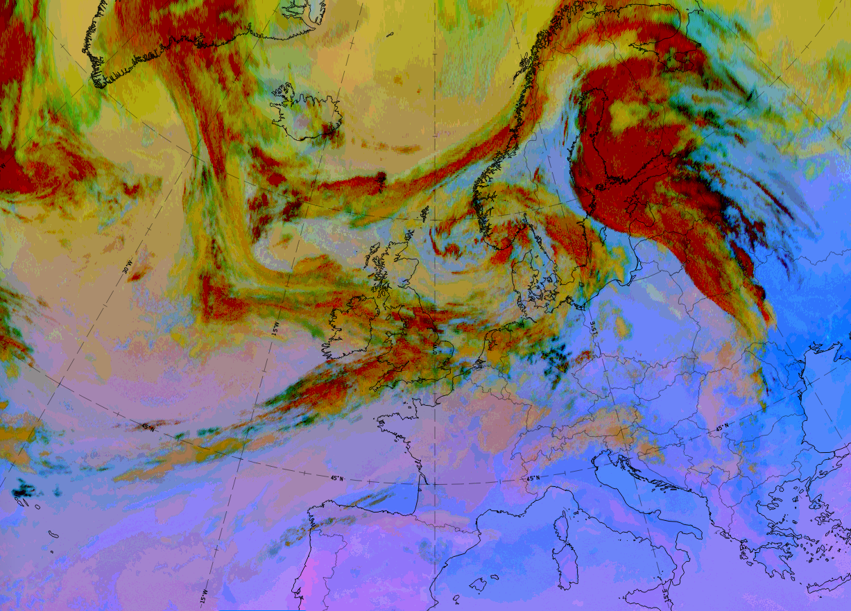
Appearance in the basic RGBs:
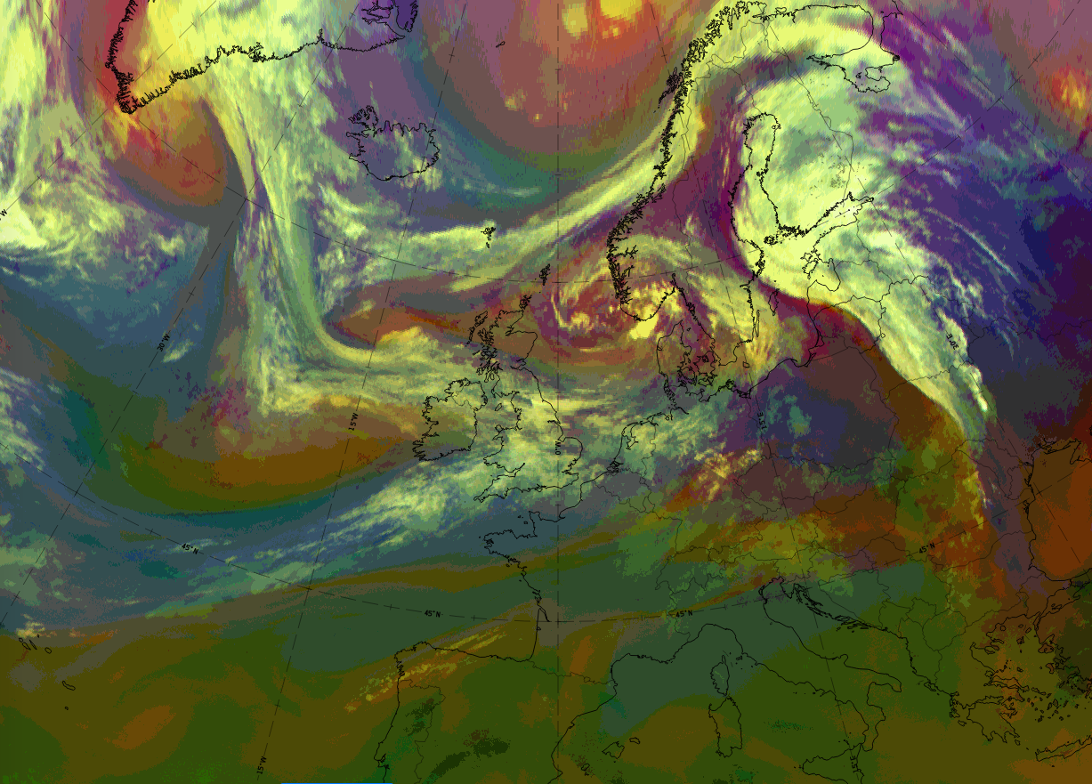
Airmass RGB
During the transition of the cloud band from an occlusion to a Back Bent Occlusion brown and dark-brown areas, representing cold and dry air, appear and intensify on both sides of the Back Bent Occlusion cloud band. This corresponds to the process of advection of cold air on the north, north-east side.
The cloud band looks very similar to that in the IR images.
Dust RGB
Unlike other existing cloud configurations, the Back Bent Occlusion cloud band is embedded within blue colours, representing cloud-free regions, or, often in northern regions, green colours representing thin mid-level cloud.
The cloud band consists of ochre and dark-red areas, representing mid-level and thick cloud regions.
 |
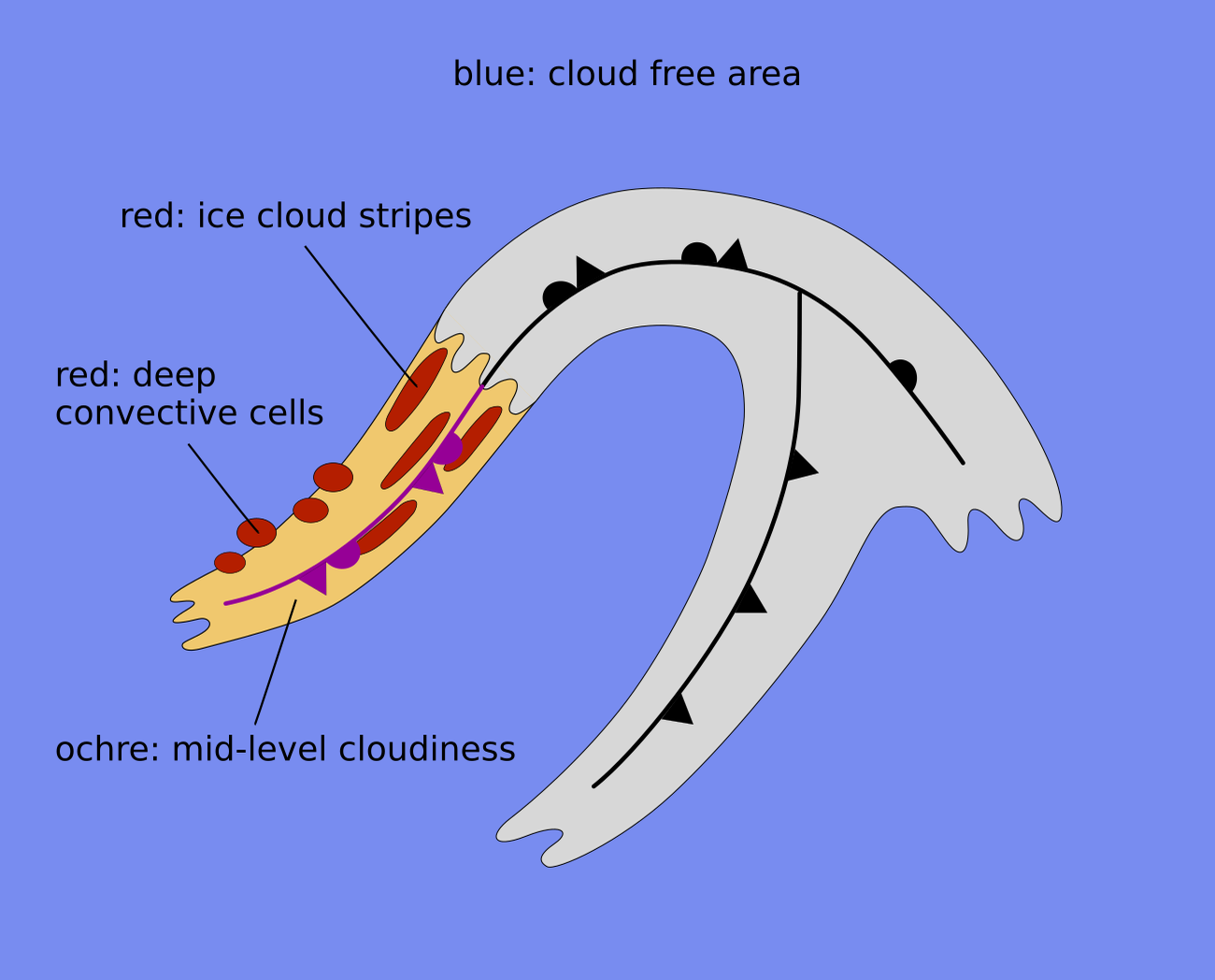 |
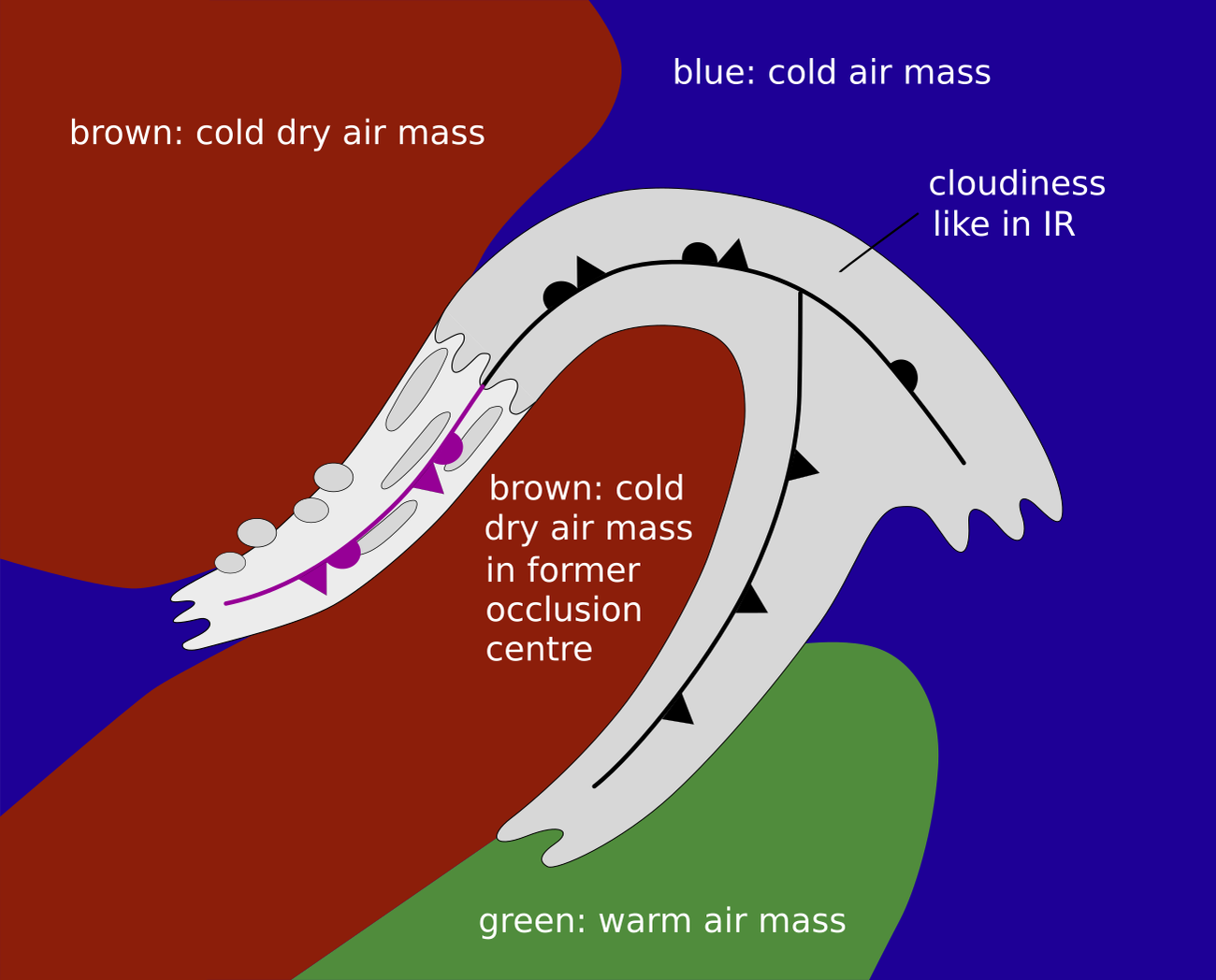
Legend: basic RGB schematics.
Left: Airmass RGB; right: Dust RGB.
The case of 29 to 30 June 2020 shows the development of a Back Bent Occlusion in the Norwegian sea. All stages from occlusion, then transition, and finally a back-bent stage, can be recognised.
On 29 June 2020 at 06 UTC, a fully developed occlusion cloud spiral extends from mid-Sweden and Norway westward across the Norwegian sea and then southward to Ireland and Scotland.
|
|


|
|
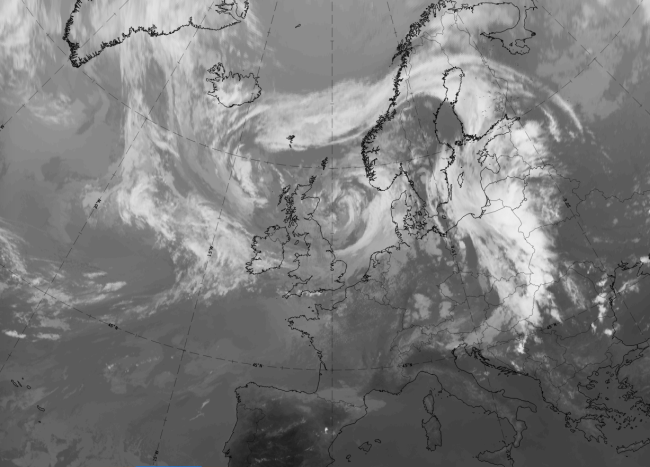
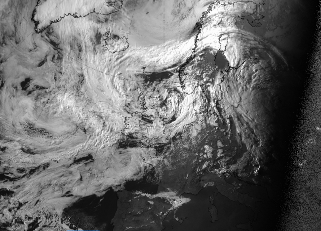
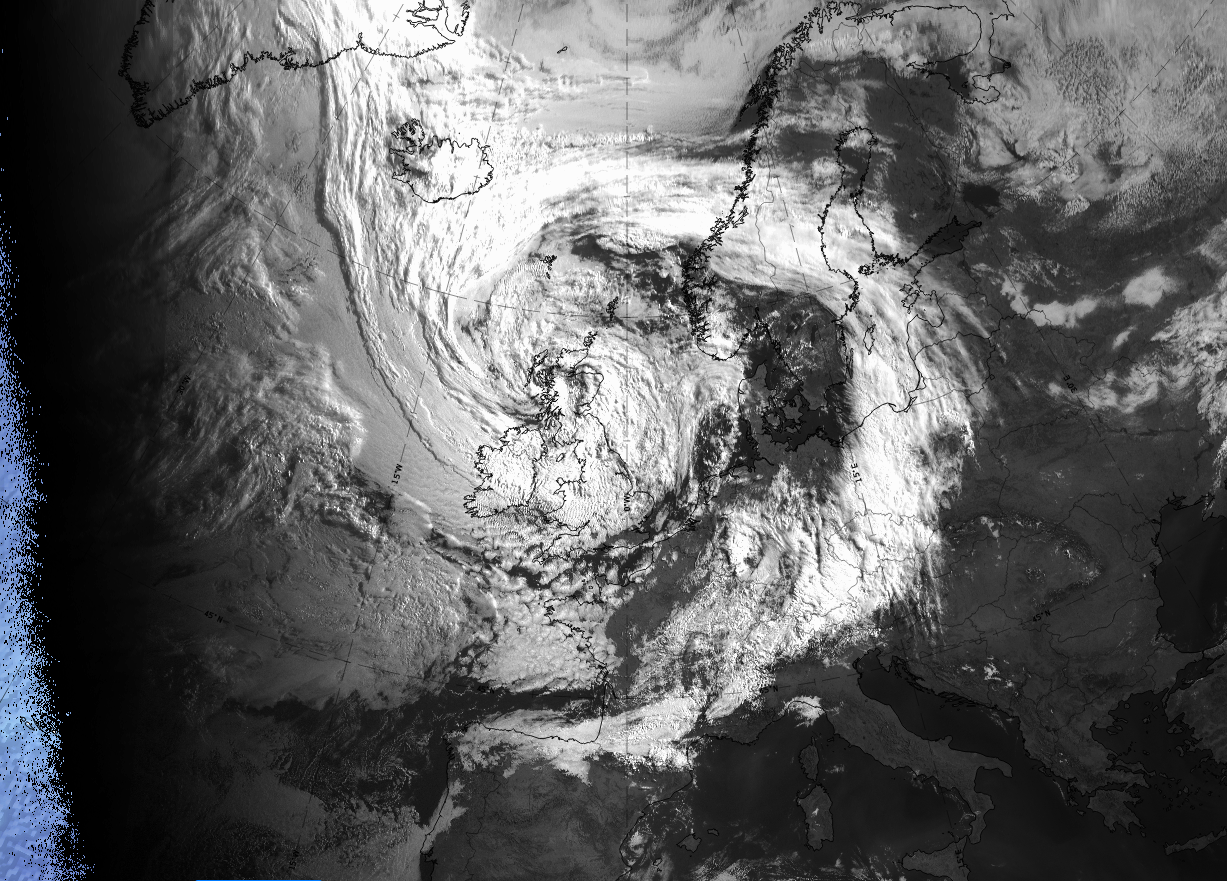
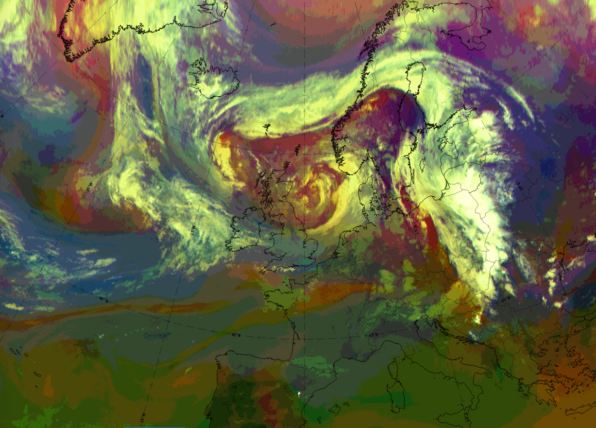
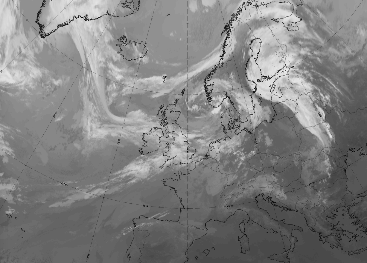
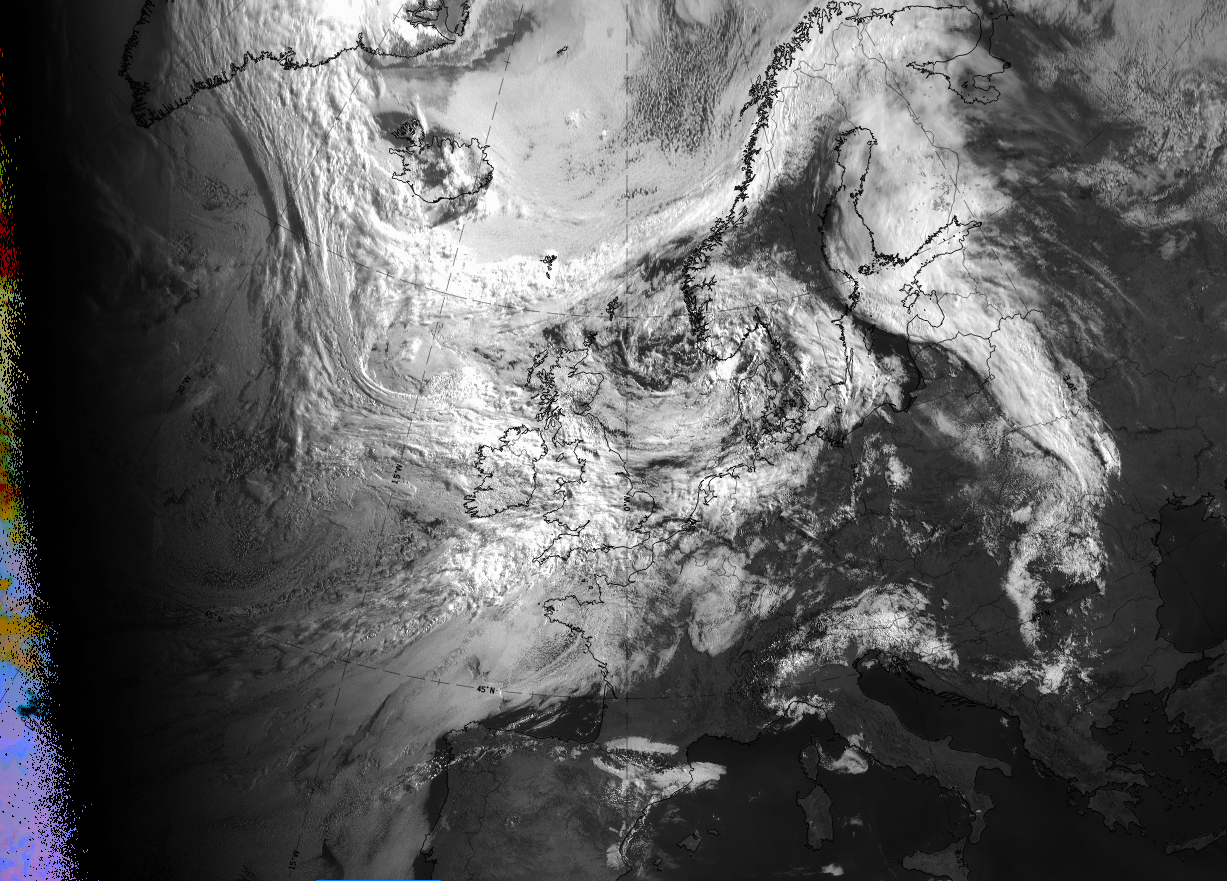
29 June 2020 at 12 UTC: "occlusion stage".
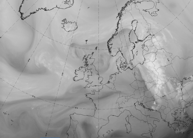
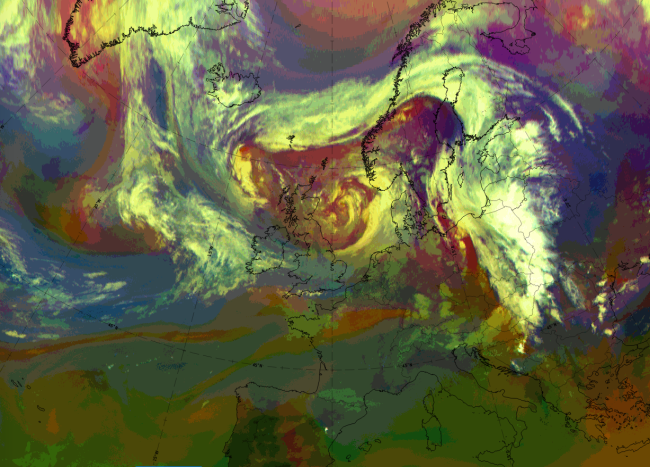
1st row: IR (above) + HRV (below); 2nd row: WV (above) + Airmass RGB (below); 3rd row: Dust RGB + image gallery.
*Note: click on the image to access the image gallery (navigate using arrows on keyboard).
On 29 June 2020 at 18 UTC, the first signs of bending back can be observed.
|
|
|
|
29 June 2020 at 18 UTC: "transition stage".
1st row: IR (above) + HRV (below); 2nd row: WV (above) + Airmass RGB (below); 3rd row: Dust RGB + image gallery.
*Note: click on the image to access the image gallery (navigate using arrows on keyboard).
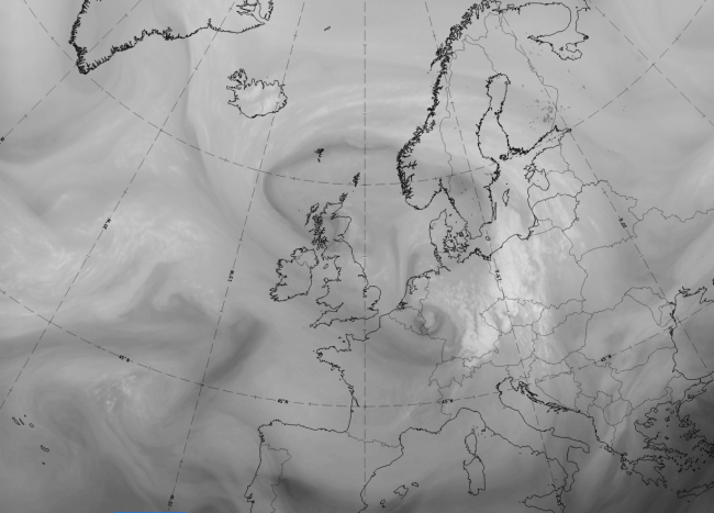
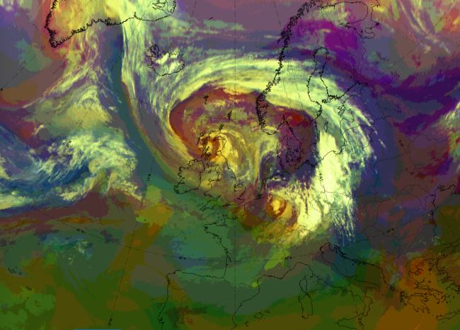
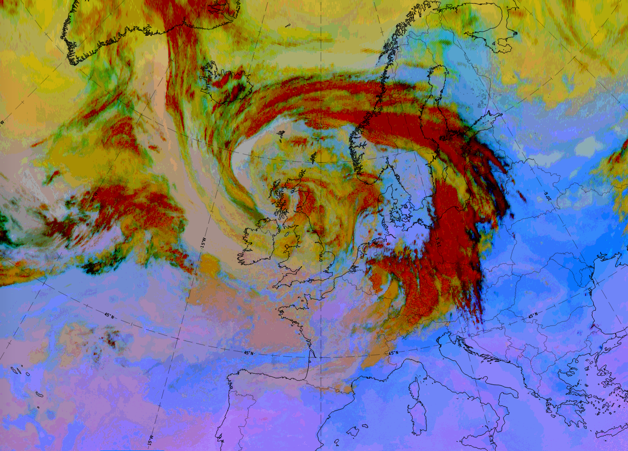
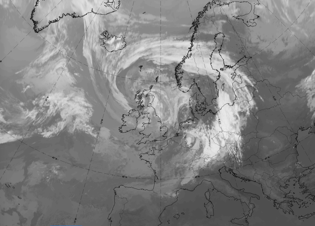
Finally, on 30 June 2020 at 06 UTC the occlusion is back-bent, showing the cyclonic curvature of a cold front.
|
|
|
|
30 June 2020 at 06 UTC: "Back Bent Occlusion".
1st row: IR (above) + HRV (below); 2nd row: WV (above) + Airmass RGB (below); 3rd row: Dust RGB + image gallery.
*Note: click on the image to access the image gallery (navigate using arrows on keyboard).
| IR | Grey and bright colours, representing at least partly thick cloud. |
| HRV | Bright colours representing partly thick cloud. |
| WV | Dark-grey and grey, representing high humidity in middle and some upper levels. |
| Airmass RGB | Dark brown colours in front of and behind the back-bent cloud band. On the south-eastern side this is the cold air in the original occlusion centre and on the north-western side this is the approaching cold air responsible for the change from occlusion to Back Bent Occlusion. |
| Dust RGB | Mostly dark red representing the thick ice cloud; the green colours to the north-west are mid-level thin cloud. |
Meteorological Physical Background
The Back Bent Occlusion can be formed, if the surface pressure gradient is relatively weak near the center of the low. The low elongates in the direction of the occluded front, and the tail of the front remains almost straight or only slightly curved; it does not curl around the low centre like in other types of Occlusions.
The bending back of an Occlusion due to cold advection
In this case there is a stationary or slowly moving low, towards which an occluded cyclone moves. They merge into each other to some extent and the cold advection from the cold side of the stationary low forces the occluded front of the cyclone to bend back.
On 18 June 2001 at 00.00 UTC there is a Warm Occlusion moving eastwards over the Atlantic. An upper low, that appears just a weak trough on the lower levels, is located west of Iceland:
| |
|

|
|
18 June 2001/00.00 UTC - Meteosat IR image; cyan: height contours 500 hPa
|
18 June 2001/00.00 UTC - Meteosat IR image; red: temperature advection 700 hPa
|
On 18 June 2001 at 12.00 UTC the lows have merged into one and there is cold advection originating from the northern side of the Iceland low affecting on the occluded front:
| |
|
|
|
18 June 2001/12.00 UTC - Meteosat IR image; cyan: height contours 500 hPa
|
18 June 2001/12.00 UTC - Meteosat IR image; red: temperature advection 700 hPa
|
On the 19 June 2001 at 06.00 UTC there is only one low left, and the cold advection has turned the occluded front into a Cold Front:
| |

|
|
|
19 June 2001/06.00 UTC - Meteosat IR image; cyan: height contours 500 hPa
|
19 June 2001/06.00 UTC - Meteosat IR image; red: temperature advection 700 hPa
|
If the cold advection is very strong, the occluded front can bend tightly as it turns into a Cold (or even into an Arctic) Front. In that case the strongest winds are connected with the new Cold Front. The area between the two Cold Fronts is sometimes called "the false warm sector":
|
The bending back of an occlusion due to a stationary high pressure area
Sometimes Back Bent Occlusions form when they approach a stationary high pressure area. A moving cyclone slows down in front of a high. The occluded front stops and bends back due to the strengthening of the high pressure centre, while the Warm and the Cold Front continue slowly within a weaker high ridge area. In this case the Occlusion can be neutral, but usually these kind of Back Bent Occlusions occur in connection with cold continental highs during the winter. There is cold advection towards the occluded front from the edge of the high pressure, and the back bent front becomes a Cold Front.
|
Relative streams
From the relative streams it can be seen that the cold air affecting the Occlusion originates from behind a low pressure in the cold airmass.
The development of the Back Bent Occlusion:
- In the first stage there is a Warm Occlusion; the air within the occluded front is rising near the Occlusion point, and remains on a constant level in area of the tail.
- The Occlusion turns into a cold one, and finally it becomes a Cold Front. Behind the Cold Occlusion and the Cold Front the air is sinking.
17 June 2001/18.00 UTC there is a Warm Occlusion southwest of Iceland:
|
17 June 2001/18.00 UTC - Vertical cross section; black: isentropes (ThetaE), red thick: temperature advection - WA, red thin: temperature
advection - CA, orange thin: IR pixel values, orange thick: WV pixel values
|
17 June 2001/18.00 UTC - Meteosat IR image; magenta: relative streams 312K
|
|
|
By 18 June 2001/12.00 UTC, the Occlusion has turned into a Cold Occlusion:
|
18 June 2001/12.00 UTC - Vertical cross section; black: isentropes (ThetaE), red thick: temperature advection - WA, red thin: temperature
advection - CA, orange thin: IR pixel values, orange thick: WV pixel values
|
18 June 2001/12.00 UTC - Meteosat IR image; magenta: relative streams 312K
|
|
|
|
19 June 2001/00.00 UTC - Vertical cross section; black: isentropes (ThetaE), red thick: temperature advection - WA, red thin: temperature
advection - CA, orange thin: IR pixel values, orange thick: WV pixel values
|
19 June 2001/00.00 UTC - Meteosat IR image; magenta: relative streams 312K
|
|
|
It should be noted that when a trough in the polar airmass reaches an occluded cyclone from the rear, the situation can resemble a Back Bent Occlusion in the satellite image or even on the surface chart. In case of a trough, however, the coldest air is within the trough, and the cold advection is ahead of the trough, in contrast with the Back Bent Occlusion, where the cold advection is behind the back bent front.
Key Parameters
- Height contours at 1000 hPa:
The surface pressure gradient is relatively weak near the centre of the low, and often elongated in the direction of the occluded front. - Height contours at 500 hPa:
In case of bending back of an Occlusion by a cold advection there is usually a low on upper levels in the cold airmass ahead of the Occlusion. In the case of a stationary high there is a pronounced large high pressure ahead of the Occlusion. - Temperature advection at 700 hPa:
In the initial stage there is warm advection ahead of the occluded front. When the front bends back, it turns into a Cold Front and there is cold advection behind it. If the cyclone is in very cold airmass, the temperature advections are even clearer at 850 hPa.
A Back Bent Occlusion can also be neutral if it is formed by a relatively warm stationary high, but this type is very rare. - Vorticity advection at 500 hPa and 300 hPa:
The field of vorticity advection shows at 300 as well as at 500 hPa a pronounced PVA maximum in connection with the Comma, but overrides the frontal cloud band during the merging process. The PVA maximum mostly is situated within the area of the Comma tail, which typically can be found within the left exit region of a jet streak. - Thermal Front Parameter:
The bending back of an occluded front can be seen from the curvature of TFP field around the Occlusion.
Height contours at 1000 hPa
|
18 June 2001/18.00 UTC - Meteosat IR image; magenta: height contours 1000 hPa, blue: temperature 850 hPa
|
|
|
|
Height contours at 500 hPa
|
18 June 2001/00.00 UTC - Meteosat IR image; cyan: height contours 500 hPa
|
|
|

|
The lows are merging and the occluded front becomes a Cold Front; black: absolute topography 500 hPa.
|
18 June 2001/06.00 UTC - Meteosat IR image; cyan: height contours 500 hPa
|
|
|
|
Temperature advection at 700 hPa
|
18 June 2001/00.00 UTC - Meteosat IR image; red: temperature advection 700 hPa
|
|
 |
|
Temperature advections in a Back Bent Occlusion that turns into a Cold Occlusion:
|
18 June 2001/18.00 UTC - Meteosat IR image; red: temperature advection 700 hPa
|
|
|
|
Thermal frontal parameter
Surface fronts in the final stage:
|
18 June 2001/18.00 UTC - Meteosat IR image; blue: thermal front parameter
|
|
|
|
Typical Appearance In Vertical Cross Sections
Cross sections for different types of occluded fronts are presented for example in the chapter Occlusion: Warm Conveyor Belt Type (see Occlusion: Warm Conveyor Belt Type - Key Parameters ). In this chapter only those parameters that indicate the process of bending back are mentioned.
- Isentropes:
In the beginning the isentropes show the structure of an Occlusion. It turns into a structure of a Cold Front during the process. - Temperature advection:
In the beginning the vertical structure of temperature advection shows a distribution typical for an Occlusion. If the Back Bent Occlusion turns into a Cold Front, which is the most usual case, it can be seen in the change of the distribution of temperature advection.
The process in which a warm occluded front turns into a Cold Front can be seen from a sequence of cross sections:
A Warm Occlusion:
|
17 June 2001/18.00 UTC - Vertical cross section; black: isentropes (ThetaE), red thick: temperature advection - WA, red thin:
temperature advection - CA, orange thin: IR pixel values, orange thick: WV pixel values
|
|
|
|
A Cold Occlusion:
|
18 June 2001/12.00 UTC - Vertical cross section; black: isentropes (ThetaE), red thick: temperature advection - WA, red thin:
temperature advection - CA, orange thin: IR pixel values, orange thick: WV pixel values
|
|
|
|
A Cold Front:
|
19 June 2001/06.00 UTC - Vertical cross section; black: isentropes (ThetaE), red thick: temperature advection - WA, red thin:
temperature advection - CA, orange thin: IR pixel values, orange thick: WV pixel values
|
|
|
|
Weather Events
| Parameter | Description |
| Precipitation | Moderate rain ahead of the warm occluded front near the low, elsewhere moderate to light rain or drizzle. Showers behind the cold occluded front. |
| Temperature | A decrease in the temperature behind the cold occluded front. |
| Wind (incl. gusts) | Possibly strong and gusty winds behind the cold occluded front. |
| Other relevant information | - |
For demonstration of weather the back-bent occlusion at 30 June 2020 at 06 UTC is chosen.
|
|
|
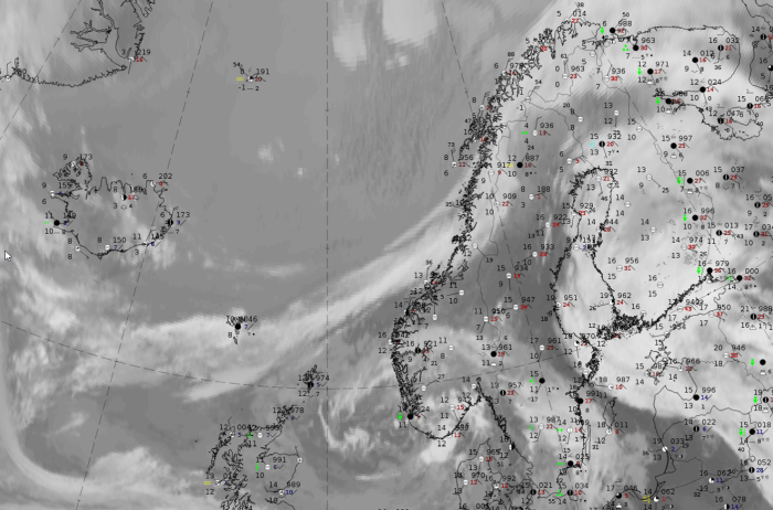
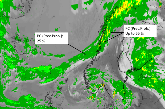
Legend:
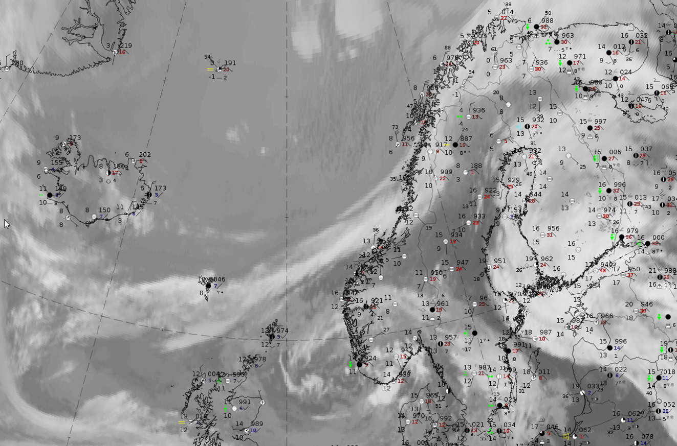
30 June 2019 at 06 UTC: IR + synoptic measurements (above) + probability of moderate rain (Precipitting clouds PC - NWCSAF).
Note: for a larger SYNOP image click this link.
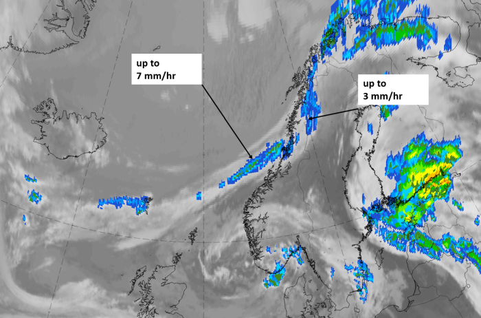
Synoptic measurements are only available for the occluded part near the former low centre. This is over North-Norway and North-Finland. The observations show precipitation not in shower form and precipitation probabilities from the NWCSAF are high there. For the back-bent part of the occlusion which extends from the Norwegian coast westward across the Norwegian Sea where there are no synoptic observation stations available the precipitation probabilities are much lower, but (this can be seen in the next figure) the convective rainfall rate determined from the NWCSAF is higher in this part than to the northeast. This corresponds with synoptic symbols in the schematic.
|
|
|
|
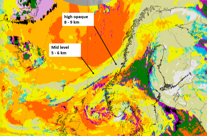
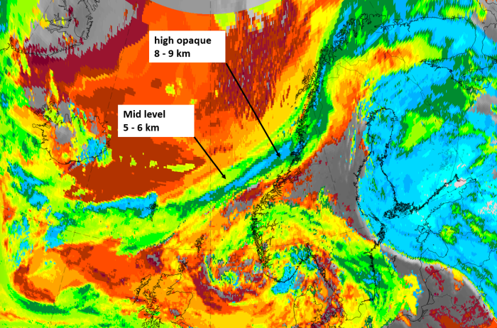
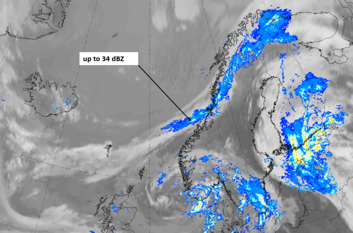
30 June 2020 at 06 UTC;
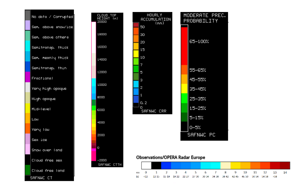
1st row: Cloud Type (CT NWCSAF) (above) + Cloud Top Height (CTTH - NWCSAF) (below); 2nd row: Convective Rainfall Rate (CRR NWCSAF) (above) + Radar intensities from Opera radar system (below).
For identifying values for Cloud type (CT), Cloud type height (CTTH), precipitating clouds (PC), and Opera radar for any pixel in the images look into the legends. (link).
References
General Meteorology and Basics
- KOISTINEN J.: Lectures on Synoptic Meteorology in the University of Helsinki, unpublished paper
- KURZ M.: Synoptic Meteorology; Deutscher Wetterdienst 1998
General Satellite Meteorology
- BADER M. J., FORBES G. S., GRANT J. R., LILLEY R. B. E. and WATERS A. J. (1995): Images in weather forecasting - A practical guide for interpreting satellite and radar imagery; Cambridge University Press.
Specific Satellite Meteorology
- The Life Cycles of Extratropical Cyclones (1999)
- A Planetary-Scale to Mesoscale Perspective of the Life Cycles of Extratropical Cyclones p. 139-161 (Shapiro, Wernli, Bao, Methven, Zou, Doyle, Holt, Donald-Grell, Neiman)
- Mesoscale Aspects of Extratropical Cyclones: An Observational Perspective p. 265- Browning (University of Reading)