Scatterometers
Scatterometers are active remote sensing instruments for deriving wind direction and speed from the roughness of the sea. They are used by low Earth orbiting satellites and act like radars: they transmit electromagnetic pulses and detect the backscattered signals. Spaceborne wind scatterometry is an indirect method of measurement. It has become an increasingly important tool for monitoring climate, forecasting (marine) weather and studying the atmosphere-ocean interactions.
Scatterometers measure the radar cross section of the ocean surface. A Geophysical Model Function (GMF) provides the radar cross section as a function of the equivalent neutral wind vector at 10 m anemometer height (not the actual wind!), incidence angle, relative azimuth angle, radar frequency, and polarization.
Depending on the wavelength of the radiation a distinction can be made between C-band and Ku-band scatterometers. The two radar types are compared with each other in Table 2. The wavelength of the radar is chosen according to the sampling scale. Thus, Ku-band radars with a wavelength of about 2 cm are sensitive to rain.
Table 2: Comparison of C-band and Ku-band scatterometers.
| C-band | Ku-band | |
|---|---|---|
| Frequency | 5.255 GHz | 13.4 GHz |
| Wavelength | 5 cm | 2 cm |
| Limitations | less detection in the higher wind range (> 60 kt), sea ice, coastal coverage - Land contamination | sensitive to rain, coastal coverage - Land contamination |
| Scatterometer | ASCAT-A and ASCAT-B | QuickScat/RapidSCAT/HY2A |
| Polarization | VV-pol | Dual-polarization |
| Sampling | 12.5-25 km | 25 km- 50 km |
| Geometry | Static | Rotating antenna |
| Swath | Double (about 550km each) | Single |
History
During World War 2 it was discovered that radars also picked up some kind of clutter over the oceans. It took some 20 more years to discover that this noise was related to wind velocity. Scatterometry started in the 1970s – the first satellite with a scatterometer onboard was Seasat-A (NASA). However, widespread usage of scatterometers started in the 1990s. Nowadays scatterometer data is operationally used especially for data assimilation and for marine nowcasting.
Figure 8 shows an overview of the current and proposed satellite missions carrying scatterometers.

Figure 8: Overview of finished, current and proposed satellite missions with scatterometeres onboard. The only exception is 'RapidSCAT', which is a scatterometer on the international space ship (ISS). (Source: http://ceos.org/ourwork/virtual-constellations/osvw/).
Backscatter
Scatterometers are radars and send pulses of radiation at the surface. The backscattered signal varies according to the wind speed and its effects on ocean roughness. Higher friction velocity means higher roughness of the sea, and thus a stronger backscattered signal. It is important to know that scatterometers are not sensitive to large (tidal) waves, but only to the wind-driven centimeter-scale capillary waves. These ripples are superimposed on the larger waves.
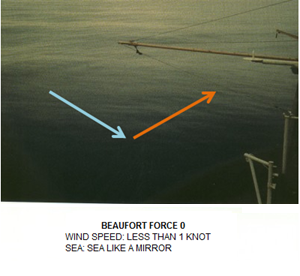

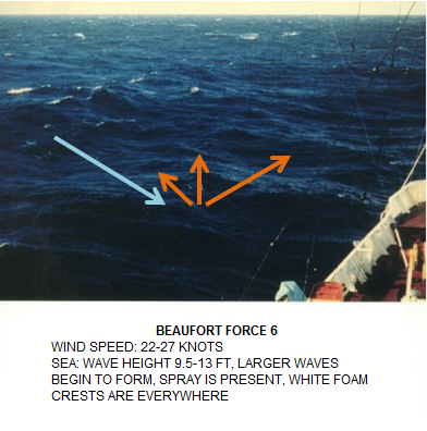
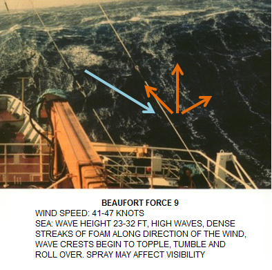
Figure 9: Bragg scattering in different Beaufort classes and therefore different states of the sea. Blue arrows show the incoming radar beam, red arrows the scattered radiation.
The scattering mechanism that occurs when electromagnetic radiation and water waves interact with similar wave lengths is called Bragg scattering. The Bragg scattering explains the effects of the reflection of electromagnetic waves on periodic structures whose distances are in the order of the wavelength.
Unlike with a flat surface, radiation is scattered in all directions rather than just being reflected. Only this Bragg scattering makes it possible to derive wind speed and direction as it changes the total amount of energy that returns to the satellite.
Bragg scattering is dependent on the incidence angle. This means that there is an optimal range of the incidence angle for scatterometer measurements. Typically angles between 30° and 60° are used as they provide the largest sensitivity to changes in wind speed. The design of scatterometers takes these facts into account which means that scatterometers only see the ocean surface from the side, never directly from above.
In Figure 9, Bragg scattering is shown for different states of the sea. The surface roughness modulates the backscattering. When the sea is glassy like at Beaufort force 1, the radar beam hardly scatters at all and merely bounces off the surface. The radar beam is refracted and keeps going. Only a small proportion is reflected back to the instrument. As the wind picks up and the waves get higher, more and more energy is reflected back to the scatterometer.
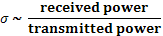
Ultimately the scatterometer measures the backscattered and normalized radiation from an extended target area (wind vector cell) sigma naught σ0.
Geophysical Model Function (GMF)
The (semi-)empirical GMF compares ocean surface wind speed and direction to the backscatter cross section measurements. The geophysical parameter that should be estimated is the wind vector. For ASCAT measurements, three known values of sigma naught are available and two unknown values - wind speed and wind direction - have to be determined. The GMF is a function of several variables:
σ0model = GMF (U10N, θ, φ, ρ, λ)
U10N ... equivalent neutral wind speed (wind at 10 m height for given surface stress assuming the marine boundary layer is neutrally stratified)
θ ... incidence angle
φ ... wind direction with respect to the direction of the radar beam
ρ ... radar beam polarization
λ ... microwave wavelength
The dependency on the azimuth angle allows determining not only the wind's speed but also its direction. Using multiple observations from different azimuth angles improves the accuracy but a minimum of two observations is required.
Scatterometer instruments
By measuring the backscattered signal by the ripples and waves, scatterometers derive wind direction and speed from the roughness of the sea. The backscattering is dependent on the incidence and azimuth angles: the dependence on the incidence angle helps to derive wind speed, while the dependence on the azimuth angle allows deriving wind direction. Two kinds of instruments are used for this measuring principle:
- fan beam scatterometers (ASCAT)
- rotating pencil beam scatterometers (RapidSCAT)
Ad 1.:
ASCAT is a so-called fan beam scatterometer. This instrument is a radar with vertically polarized antennas. It consists of two sets of three antennas. Thus each point of the surface is seen and measured by the scatterometer three times. The radar beams are directed 45 degrees forward, orthogonally, and 45 degrees backwards relativ to the satellite's flight direction, on both sides of the satellite ground track (see Figure 10). Each scanning swath has a width of 550 km with a scanning gap of 670 km in between (see Figure 11). This scanning gap is a result of the optimal incidence angle of Bragg scattering. The antenna structures are typically about three meters in length and require large unobstructed fields of view on the spacecraft. Due to the antenna geometry, different measuring points on the surface have different incident angles.
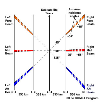
Figure 10: Antenna design of a fan beam scatterometer.
Each beam provides measurements of radar backscatter on a 12.5 km and/or 25 km grid, in such a way that each swath is divided into 41 (41*12,5) or 21 (21*25) so-called Wind Vector Cells (WVCs). Each WVC is viewed thrice because of the three different viewing directions caused by the antenna geometry. Thus one obtains three independent backscatter measurements - triplets of sigma naught σ0 - separated by a short time delay. A mathematical model ("Geophysical Model Function" GMF) is then used for deriving wind speed and wind direction on the ocean surface out of the triplets of sigma naught.
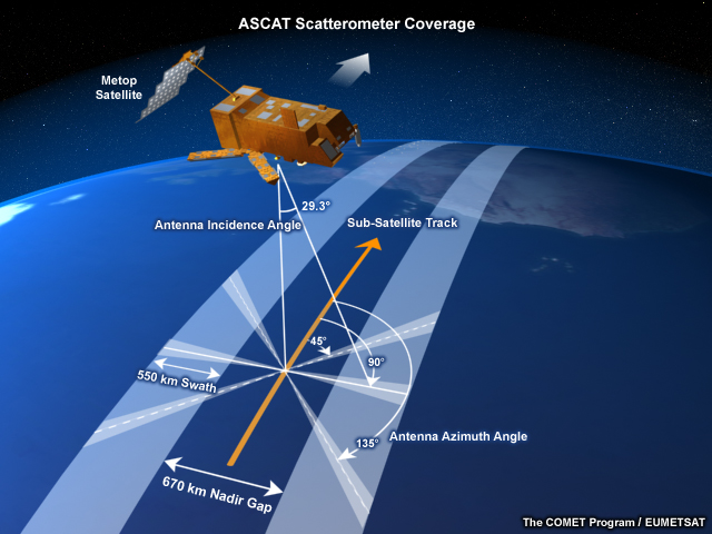
Figure 11: Measuring geometry of a fan beam antenna onboard of ASCAT.
The ASCAT fan beam instrument operates at a frequency of 5.255 GHz (C-band). This makes it fairly insensitive to rain, but C-band radars have limitations when it comes to extreme wind speeds larger than 60 knots.
Ad 2.:
The rotating pencil beam scatterometer uses a rotating radar. The radar emits signals at certain incidence angles. It never looks directly beneath the spacecraft as those incidence angles are not suitable for deriving wind speed and direction. The radar sends out two rotating beams with different polarizations (vertical and horizontal). For example RapidScat, the scatterometer which is on the ISS, scans at an incidence angle of 49 degrees for the inner beam (horizontal polarisation) and 56 degrees for the outer beam (vertical polarization) as shown in Figure 12. These two polarisations have slightly different backscatter characteristics and thus the quality of wind speed and direction estimations is improved.
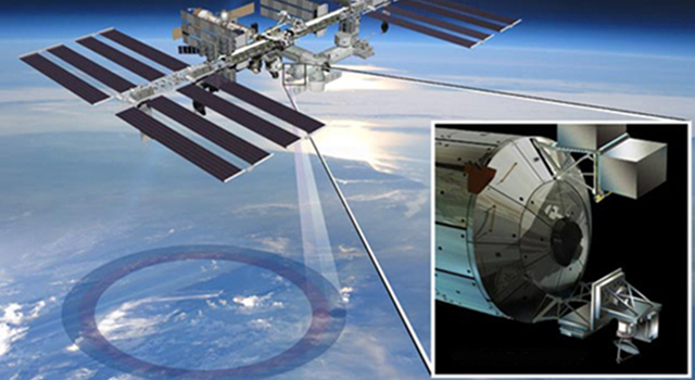
Figure 12: The working method of RapidScat as an example of rotating pencil beam scatterometers (image source: www.nasa.gov/Rapidscat).
Figure 13 shows the measurement geometry of a rotating pencil beam scatterometer. The two different incidence angles and the different polarizations allow a very precise determination of wind speed and direction. Each footprint on the ocean surface is observed twice: when it is located in front and behind the satellite track. Thus up to four observations of the same spot are made in the mid-swath when horizontally and vertically polarized beams are considered individually (see Figure 13). In the far-swath, only the vertically polarized beam provides surface observations. The best quality of measurements can be obtained in the mid swath due to good azimuth diversity.
Measuring backscatter with the help of a rotating pencil beam scatterometer has two advantages over the fan beam scatterometer: first, due to its compact design it is much easier to accommodate on satellites or spacecrafts. Second, no 'nadir-gap' appears. However, due to the poor azimuth diversity the measurements in the nadir swath may not be unambiguous.
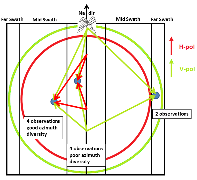
Figure 13: Measurement geometry of a rotating pencil beam scatterometer (Source: J. Sienkiewicz).
Wind retrieval algorithm
Several steps are needed to convert the measurements of sigma naught into wind data:
- NWP collocation: first, land and sea ice regions have to be excluded from the wind retrieval areas
- Quality control: the sigma naught values are quality checked
- Wind computation by GMF inversion: the Geophysical Model Function (GMF) is used for converting the sigma naught values to wind speed and direction. The GMF has an empirical or semi-empirical form.
- Field-wise ambiguity removal: each wind vector cell has four possible solutions for wind direction and speed. The correct solution is determined by using NWP forecasts and wind field spatial patterns.
Limitations
In general, the quality of scatterometer winds is quite good. But there are some situations where the data can be compromised:
- sea ice and land contamination (see Figure 14)
- large spatial wind variability (for example in the vicinity of fronts and low pressure centers, e.g. downbursts)
- rain - especially in Ku-band systems (see Figure 15)
- higher wind speeds (>60 knots) - especially in C-band systems
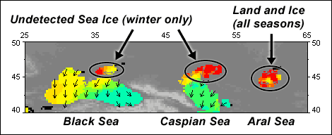
Figure 14: Example for sea ice and land contamination from the QuikScat scatterometer (source: http://www.remss.com/missions/qscat).
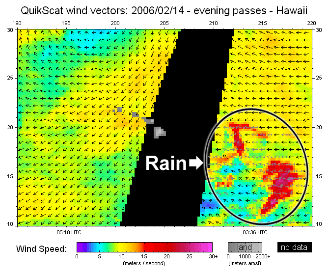
Figure 15: Example for rain contamination from the QuikScat scatterometer (source: http://www.remss.com/missions/qscat).
Rain effects
Ku-band scatteromenters are particularly sensitive to rain. For C-band scatterometeres the rain effects are less significant.
- radar signal and the backscattered information are attenuated by rain
- - σ0 and the retrieved wind speed decreases
- radar signal is scattered by the rain drops
- - σ0 and the retrieved wind speed increases and directional information can be lost
- the roughness of the sea surface is increased due to the splashing of rain drops - this effect mainly occurs at low wind speeds when the sea surface is calm
- - σ0 and the retrieved wind speed increases
- - directional information may also be lost
- variable roughness of the sea surface due to wind downbursts and/or a gust front
- - confused sea state: wind speed and direction might be unclear
- - area influenced by the downburst might be bigger than the area affected by the splashing of rain
Rain contaminated winds can be detected in the majority of cases as those wind vectors are oriented perpendicular to the satellite's track. Rain also increases wind speed most of the time.