Training Module on Monitoring Vegetation From Space

4 - Empirical Vegetation Indices

Vegetation indices (VI's) have a long history of use over a wide range of applications, such as vegetation monitoring; climate and hydrologic modelling; agricultural activities; drought studies and public health issues. As shown in chapter 3, vegetation has unique spectral signatures, which evolve with the plant life cycle. VI's are dimensionless radiometric measures, which combine information from different channels, particularly in the red and NIR portions of the spectrum, to enhance the 'vegetation signal'. Such indices allow reliable spatial and temporal inter-comparisons of terrestrial photosynthetic activity and canopy structural variations. They are generally computed for all pixels in time and space, regardless of biome type, land cover condition and soil type, and thus represent true surface measurements. Due to their simplicity, ease of application, vegetation indices have a wide range of usage within the user community.

4.1 - NDVI

As detailed in chapter 3, the relationship of red and NIR reflected energy is clearly related to the amount of vegetation present on the ground (Huete et al. 1999). Reflected red energy decreases with plant development due to the chlorophyll absorption within actively photosynthetic leaves. Reflected NIR energy, on the other hand, will increase with plant development through scattering processes in healthy leaves.

The most widely used VI is the Normalized Difference Vegetation Index, it consists of a normalized ratio of the NIR and red bands

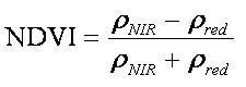
Where:

ρ_red and ρ_NIR (either top of atmosphere or surface bidirectional) are the reflectance measurements for VIS red and NIR bands, respectively.

For land targets the index ranges from values close to 0 for arid or barren areas to ~ 1 for densely vegetated areas. Negative values of NDVI usually correspond to urban areas. The NDVI over water surfaces is very close to -1 due to their very low reflectance in the NIR band.

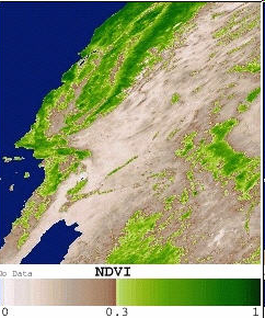
Figure 4.1: MODIS/Terra Vegetation NDVI 16-Day L3 Global 250m SIN Grid.

NDVI main advantages and disadvantages.

Advantages:

• As a simple transformation of spectral bands, NDVI is easily computed without assumptions regarding land cover classes, soil type or climatic conditions
• Long time series (more than 20 years) available.

Disadvantages:

• Inherent nonlinearity because it is a ratio based index
• Additive noise effects
• Asymptotic (saturated) signals over high biomass conditions
• Very sensible to canopy background brightness (Huete, 2002)
• Is not a structural property of a land surface areas

4.2 - EVI

The Enhanced Vegetation Index was developed by the MODIS Science Team to take full advantages of the sensor capabilities. In order to increase the sensitivity to the vegetation signal, the index makes use of measurements in the red and near infrared bands (as in the case of NDVI), and also in the visible blue band, which allows for an extra correction of aerosol scattering. EVI also performs better than NDVI over high biomass areas, since it does not saturate as easily.

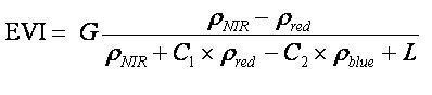
Where ρ are atmospherically corrected or partially corrected (Rayleigh and ozone absorption) reflectances, L is the canopy background adjustment, C₁ and C₂ are coefficients related to aerosol correction and G is a gain factor. The blue band is used to remove residual atmosphere contamination caused by smoke and sub-pixel thin clouds

Figure 4.2: MODIS/Terra Vegetation EVI 16-Day L3 Global 250m SIN Grid.

EVI main advantages and disadvantages.

Advantages:

• Found to perform well under high aerosol loads , biomass burning conditions (Huete et al., 2002)

Disadvantages:

• Inherent nonlinearity because it is a ratio based index
• To compensate for the effects of NDVI saturation over high biomass areas, EVI tends to present relatively low values in all biomes and also lower ranges over semiarid sites.
• The correction for aerosol impact on the final index makes use of reflectances measurements within VIS blue, not always available (the case of AVHRR or SEVIRI sensors).
• Is not a structural property of a land surface areas

4.3 - EVI vs NDVI performance and common drawbacks

Figure 4.3: NDVI vs EVI performance

A problem common to all VI's is their empirical nature. These two figures show the steep gradient in vegetation cover over South America, including: the hyperarid Atacama desert (no vegetation), the semi-arid and sub-humid portions of the Brazilian Cerrado (savannah biome), and the humid and perhumid portions of the Amazon tropical rainforest.

4.4 - Other vegetation Indices

Several other vegetation indices have been developed for different sensors and with different purposes:

• Perpendicular Vegetation Index (PVI)
  

  

• Soil Brightness Index (SBI)
  

  

• Green Vegetation Index (GVI)
  

  

• Vegetation Condition Index (VCI)
  

  

4.5 - Applications

VIs are widely used to assess how environmental changes affect the distribution and dynamics of vegetation, particullarly at large temporal and spatial scales, and/or in areas of limited in situ data. In this chapter we will present examples of NDVI use to assess environmental consequences of DROUGHT:

• Vegetation stress
• Crop monitoring

4.5.1.Drought Monitoring

Drought and vegetation stress in Portugal 2004

The strong dependence of vegetation dynamics on water availability has been for long recognized in semi-arid regions (Gouveia et al. 2009). Under such conditions VI's can be used to identify areas prone to drought. However VI's must be used carefully. For example low values of NDVI indicate bare/low vegetated areas, but NDVI by itself cannot be considered a drought index since the concept of drought implies an extreme condition and a deviation from normal status. In terms of vegetation dynamics, a drought is an event that hampers the normal vegetation growth. In order to capture this effect, and to compare drought conditions in areas with different land cover, NDVI information has to be complemented with climatic information.

Next figure presents monthly NDVI anomalies for September 2004 - to - August 2005, defined as departures from the respective monthly medians. The latter statistics were obtained from NDVI time-series encompassing the September 1998 - to - July 2006 period, and derived from VEGETATION instrument onboard SPOT 4 and SPOT 5 (Gouveia, C. et al. 2009).

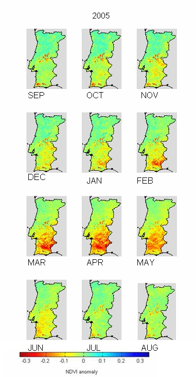
Figure 4.4: NDVI monthly anomalies between September 2004 and August 2005 derived from images acquired by the VEGETATION instrument onboard SPOT 4 and SPOT 5 (Gouveia et al. 2009).
(*) - During the summer season of 2005, Portugal was also hit by large wild fires. You can learn further details about this Fire event at the Forest Fires EUMETRAIN CAL Module

Drought and Crop production decrease in Kenya 2009

The amount of precipitation of Kenyas 2009 "long rains" season was well below the climatological average and also under the 2008 "long rains", which was also a dry year. The figure shows the MODIS NDVI 16-day composite for the period between Sep 14 and Sep 29 in 2007 (left panel) and in 2009 (right panel).

The figure shows the MODIS NDVI 16-day composite from Sept 14 until Sept 29 for 2007 on the left and for 2009, on the right.

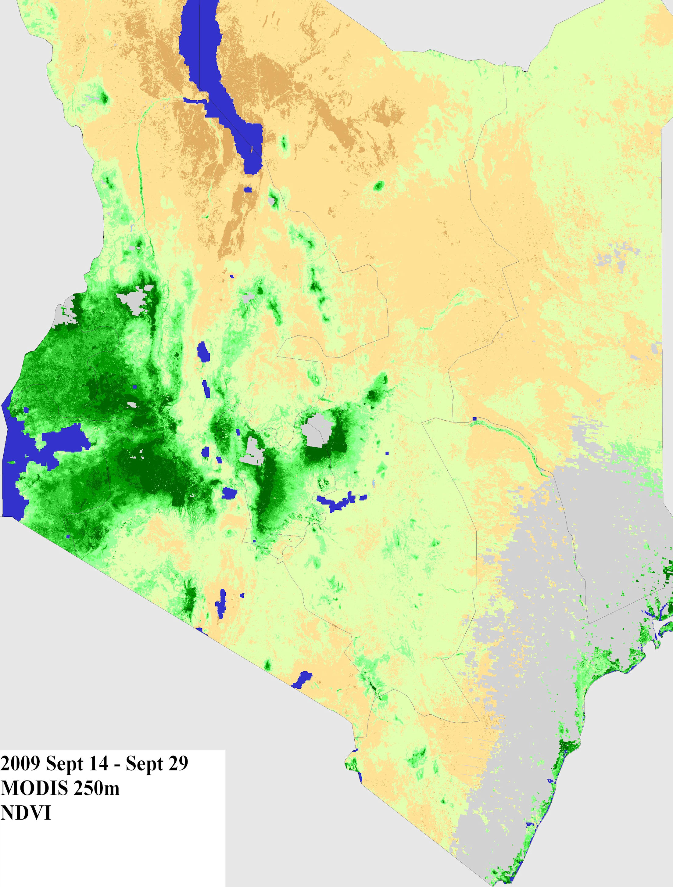
Figure 4.5: NDVI 16-day composite for Sep 14 - Sep 29 2007(left) and the same period in 2009 (right) derived from MODIS 250m spatial resolution.

The 2009 NDVI shows a dramatic decrease of vegetation dynamics when compared with 2007. Because NDVI correlates well with relative grain yields for most agro-climates in Kenya (USDA FAS - Commodity Intelligency Report, Dec 2009), the comparison of 2007 and 2009 NDVI suggests that the severe 2009 drought will reduce the Kenya's 2009 "long rain" corn yields. In fact USDA's Foreign Agricultural Service forecasted for Kenyas 2009/10 corn production 1.8 million tons, down 0.3 million tons compared to the previous year already poor crop and considerably less than the 5-year average of 2.6 million tons. We will return to this subject latter on this module section 5.9.3.