5.5 - Algorithms
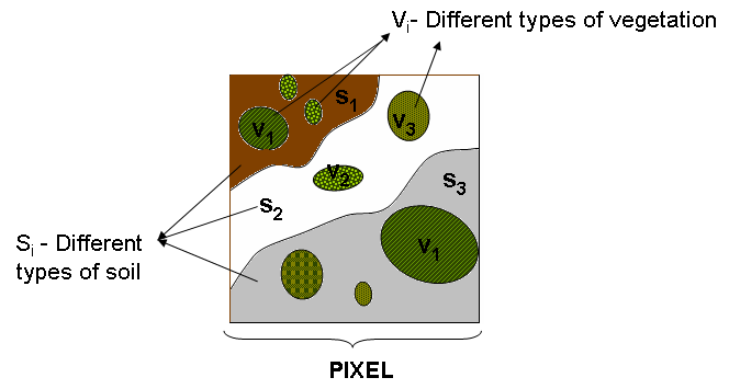
The retrieval of FVC, LAI and fAPAR in the LSA SAF rely on Spectral Mixture Analysis (SMA); the signal from a single pixel (surface reflectance) is assumed to be the contribution of different vegetation and bare soil components within the scene (next figure).
As detailed in Chapter 2, the surface BRDF may be written as:
ρ (θs, θv, φ) = K0 + K1 x F1(θs, θv, φ) + K2 x F2(θs, θv, φ)
Where:
K0 - represents isotropic reflectance;
K1 - represents geometric reflectance;
K2 - represents volumetric reflectance;
Parameters K0 in the SEVIRI channels VIS 0.6 μm, VIS 0.8 μm and NIR 1.6 μm are used to determine FVC and LAI, while fAPAR uses K0, K1 and K2.
5.5.1 - LSA SAF FVC
The estimation of FVC is based on the analysis of K0 for VIS 0.6 μm, VIS 0.8 μm and NIR 1.6 μm channels. The K0 component of surface reflectance is the less affected by shadows and, therefore is able to provide a physically correct estimation of FVC. Taking into account the spectral signature of pure types of vegetation (V1,V2,V3) and soil (S1,S2,S3), the SMA process allows to estimate the fraction of the vegetation types present in the pixel.
Next figure shows an example, considering a 2 dimensional space [0.8 μm K0 and 0.6 μm K0 ]
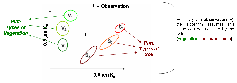
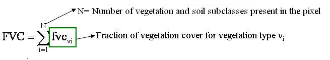
Therefore FVC is estimated by the following expression:
Pure vegetation types consider species prevalent in:
- V1 - Crops
- V2 - Herbaceous ecosystems
- V3 - Forest
Soil types include:
- S1 - Bare soil
- S2 - Rock
- S3 - Human-built surfaces
Next figure shows an example of FVC over the Full SEVIRI disk (figure on the left), and the corresponding Error (figure on the right) for the 15th April 2007.
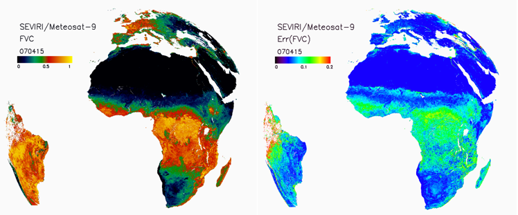
The FVC image adequately captures the spatial patterns of vegetation cover at continental level. Large spatial variation gradients are observed over Africa. This figure also highlights the spatial homogeneity and the absence of large gaps in the FVC field.
5.5.2 - LSA SAF LAI
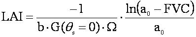
LAI in the LSA SAF is retrieved using a semi-empirical method proposed by Roujean and Lacaze (2002), in which LAI is related to FVC trough the following expression:
Where:
- a0 - is a coefficient within the range 1.04 to 1.07;
- b = 0.945;
- G = 0.5;
Both coefficients a0 and Ω depend on a Land Cover Classification Map (GLC2000) GLC2000_EUR.pdf
The next figure shows an example of LAI over the Full SEVIRI disk (figure on the left), and the corresponding Error (figure on the right) for the 15th April 2007.
Large spatial gradients of LAI are also found over Africa:
- LAI ~ 0 on the Sahara desert;
- LAI gradually increases in the Sahel from areas with sparse vegetation to woody Savannas, reaching the highest values in the equatorial forests;
- In the southern hemisphere, LAI decreases again from tropical forest through the woody savannas to the desert of Namibia;
- The higher values within the Meteosat disk (LAI= 6.5) are found in Amazonian forest.
5.5.3 - LSA SAF fAPAR
The fAPAR is estimated from a NDVI-like vegetation index, the RDVI (Renormalized Difference Vegetation Index).
As you have seen, in chapter 4, NDVI is given by the normalized difference between reflectances in channels 0.6 μm and 0.8 μm. RDVI, is a very similar parameter given by:

RDVI has a behaviour close to that of NDVI for large LAI, but tends to be more sensitive to changes in vegetation coverage under low LAI conditions. Since the view-illumination geometry may have a large impact on reflectance observations, RDVI is computed using 0.6 μm and 0.8 μm surface reflectances corrected to an optimal geometry, which maximizes the correlation with fAPAR. Such corrected reflectance values are estimated, for each channel, from K0, K1 and K2 parameters (Roujean et al. 1992):
corresponding to solar and view zenith angles of 45° and 60°, respectively. fAPAR estimation explores its linear relationship to RDVI (obtained for the optimal geometry):
Next figure shows an example of fAPAR over the Full SEVIRI disk (figure on the left), and the corresponding Error (figure on the right) for the 15th April 2007.
