Vertical Profiles
In the below image the observed sounding of Palma de Mallorca is plotted.
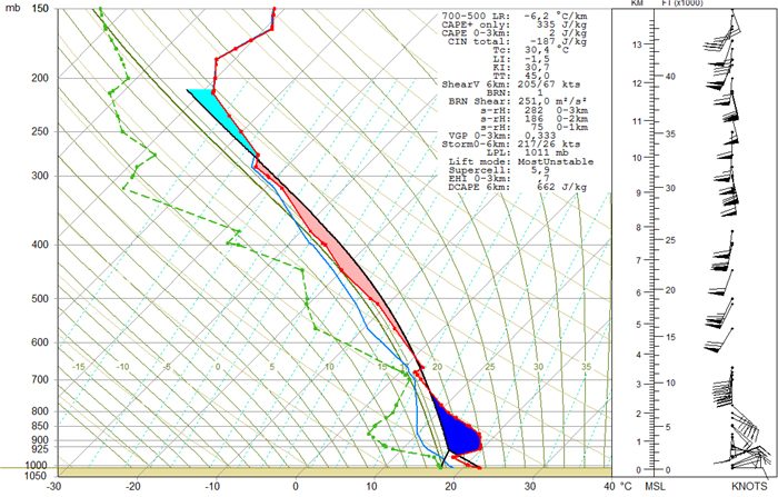
Figure 4.1: Observed sounding Palma de Mallorca. 4 October 2007 12UTC
Striking and main features are the:
- Presence of low level and deep layer shear, with a 70 kt southwesterly jet at around 5km
- Large convective inhibition, which will prevent initiation unless a significant forcing available. CIN will decrease with time as a result of low level advections. Also, a mesoscale forcing source will arrive in place at 15 UTC, as we know now, after the event.
- A shallow layer of latent instability near the ground, with no so large associated potential bouyancies (most unstable CAPE =MUCAPE=335 J/kg)
- Presence of an elevated mixed layer (EML) from 875 to 700 hpa (elevated source of African air, as pointed out in chapter 2 when the MODIS image comments)
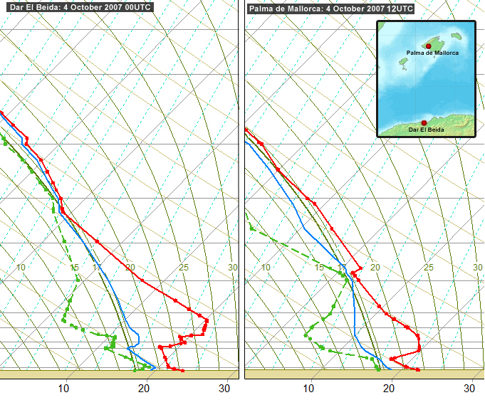
The source of the EML can be traced back and confirmed by checking the sounding from Dar El Beida in Algeria. The sounding for 4th october at 00 UTC, confirms that the EML found in Mallorca at 12UTC is advected by a southerly and mid-level flow which is directed towards the Balearic Islands.
Relevant to this and to demonstrate the performance of the model we will show you the analysis of ECMWF for 12UTC and the +3 hour forecast for 15UTC for the sounding over Mallorca Bay (39.5°N, 2.6°E)
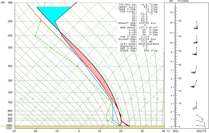
Figure 4.2: ECMWF analysis of 12UTC at Mallorca bay (39.5°N, 2.6°E). In red: temperature / green: dew point / blue: wet bulb temperature / black: most unstable parcel lifting path / 17.5 critical saturated adiabat outlined for clarification of latent instability layers
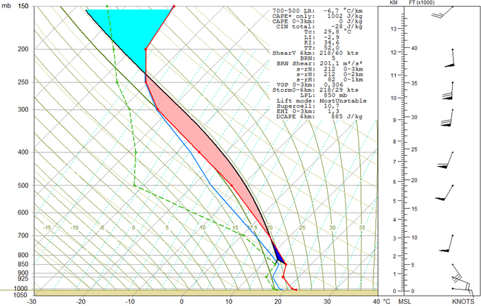
Figure 4.3: The 3 hour forecast valid for 15 UTC vertical profile at Mallorca bay (39.5°N, 2.6°E). The layer of latent instability is forecasted to increase markedly, mainly as a result of temperature and dew point advection at low levels
Regarding the three hours forecasted evolution of the vertical profile, two main features are clearly seen at low levels:
- A marked increase in depth of latent instability layer, as a result of positive advection of temperature and dew point at low levels. This is also reflected in the increase in MUCAPE value from 687 J/kg at 12 UTC to 1002 J/kg at 15UTC. Is important to stress here, that despite CAPE values are not impressive, there is a large number of parcels with moderate positive buoyancies, which is very relevant for the assesment of convection intensity.
- An increase in low level shear and helicity, as a result of the intensifying low level easterly flow, and also medium level southerly flow.
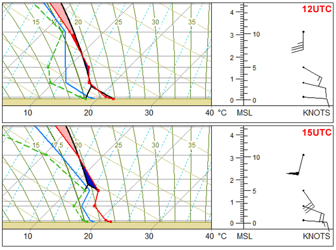
Figure 4.4: Zoom to the lower layers of troposphere. ECMWF analysis (12Z) (top) and 3 hour forecasted (15Z) soundings (bottom)
Verify that most unstable parcel at 12 UTC is at the surface, but at 15 UTC this parcel is at 850 hpa, where advections of temperature and humidity are forecasted to be larger (as a result of a marked increase of wind speed at this levels, from 15 to 30 knots).
NOTE: It should be taken into consideration that these profiles have been obtained from model output in standard pressure levels, so vertical resolution is not so high, and errors in convective parameters are to be expected. Still this model output is enough to show the main features we want to stress here.
At upper levels, we can also confirm the approaching of the jet streak from 12 to 15 UTC. The max winds are located around 9-10 km from MSL (see mesoscale analysis and forecast section). A corresponding increase in deep layer shear is also to be expected. For instance, forecasted BRN shear for 15 UTC is 202 m2 s-2, which is really a large value, implying that for convection to be sustained in this environment, a high degree of organization and intensity is required, otherwise, so much shear would be detrimental for the maintenance of convective activity.
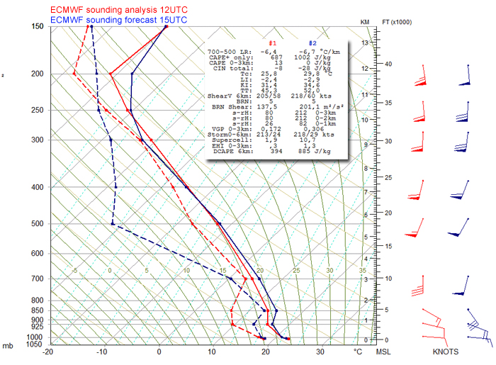
Figure 4.5: Comparison between the analysis and the three hour forecasted sounding of ECMWF.
Finally, although is not easy to interpret them for this case, we show a comparation of 12 UTC ECMWF run, analysis (left) and 3 hour forecasted (right) hodographs, at the same location as before (Lat, Lon) = (39.5N, 2.6E), and again calculated with standard pressure levels. Together with the hodographs, storm motion vector and storm relative winds are plotted.
For convective parameters computation, a storm motion vector has to be adopted, and here we follow the traditional approach, so the storm is supposed to move with 75% of mean flow speed and 30° to its right, which is not very realistic in this case, because our MCS, by 15 UTC, did not move to the right of the mean flow, even did not moved at the forecasted speed, but markedly faster.
Still, this simplified approach, give some insight on the evolution of kinematic convective parameters, that can be of use in an operational context in future cases and also, from the training perspective, we consider good idea to start using hodographs information as a side tool in the nowcasting proccess.
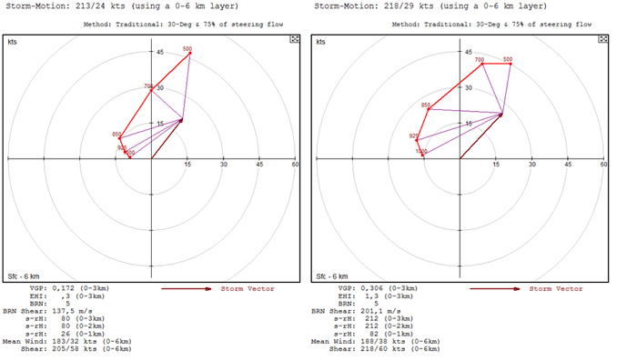
Please make note of the clockwise curvature of the hodographs, especially at low levels, in agreement with the low level warm advection, that allows for positive SRH values. Check that 3 km SRH is under-calculated by the software, because of the lack of two sampling points between 2 and 3 km height, so, obviously, a value much larger than 212 m 2 s-2 at 15 UTC should be expected. Because of similar reasons, 1 km and 2 km SRH's are also under-calculated. Regarding the 3 hours evolution of the hodograph, apart from the increase of SRH values, three other key ingredients are present:
- A marked increase in low levels storm relative flow by 15 UTC (size of the purple vectors)
- A marked increase in low level shear in layers 1000-925 and 925-850 hPa.
- A quite large streamwise vorticity at 1000 and 925 hpa (shear vector perpendicular to storm relative wind)
Allthough these three elements are considered necesary for tornadogenesis, obviously, their presence can never be taken as a predictor. Also, the environment attached to the arriving forcing source (the MCS gust front) can be quite different than the forecasted one, but this can not be assessed in this case study, because of the lack of radar derived wind information at low levels.