Appearance in cross sections
The structure of a polar low can be further studied by looking at prognostic cross sections. For comparison we consider here cross sections along line A, typical for a well mixed marine Mixed Layer (MML) and along lines B and C, across the center of the polar low. Here fields from the Norwegian Arome-Arctic 2.5km model is shown, with a forecast length of 12 hrs.
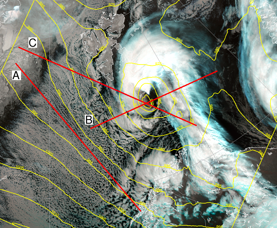
Figure 4.1: Cross sections (red lines) from the 19th January 2017, 12 utc. Yellow lines are a 12 hr. prognosis for MSLP, indicating a center at 74.5N 22.5E. Illustration: MET-Norway
Vorticity advection
One of the main dynamical mechanisms in the initial or developing phase is Positive Vorticity Advection (PVA) caused by a moving upper level through. To trigger a Polar Low, a PVA maximum has to be superimposed upon the baroclinic zone.
Potential vorticity
Potential Vorticity (PV) is an important parameter in the development phase of a Polar Low. In this stage an upper level PV maximum is normally just upstream of a Polar Low.
This PV maximum is situated at mid levels of the troposphere but has transferred down from the stratosphere. A PV maximum can also be found in the gradient zone of the very stable layer near the surface over or near icefields.
Vertical Motion
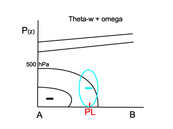
Figure 4.2: Vertical Motion (omega)
In figure 4.3 and 4.4 a stable layer is seen as horizontal isolines for the potential temperature (θ). Vertical orientation in the isolines for θ indicates a well mixed layer and a statically unstable air mass. In a cold air outbreak there is a strong inversion above the marine mixed layer. Figure 4.3 shows a cross section along line A west of the polar low. Here there is a homogenous layer of shallow convection which extends upwards to the inversion. Smaller areas of negative ω associated with individual convection cells can be seen adjacent to areas of positive ω, in the dry sinking air outside the convection cells. The absolute values of ω are of more than -3 hPa/sek, but the maxima are confined to small areas. Cumulus Congestus (often called towering Cumulus) usually have a horizontal extent of a few kilometers, but with sharp gradients between areas of ascending and descending air. For aviation, turbulence associated with TCu's are described as moderate.
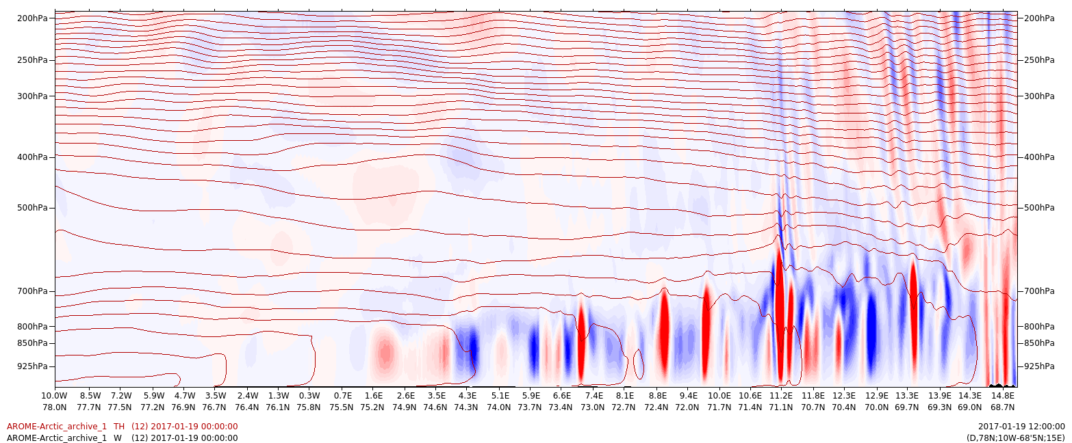
Figure 4.3: Shows potential temperature (dark red lines) and vertical speed (blue/red shading for +/- ω) along line A through the cold air outbreak to the west of the polar low. Illustration: MET-Norway
If the inversion above the MML is broken down, deeper convection can take place, and polar lows may form. A polar low will manifest itself as larger areas of ascending air and negative ω. The absolute values are similar to what can be found in more shallow convection, but the horizontal and vertical extent is larger. The negative ω is associated with the deep convection around the center of the low, in figure 4.4 seen as bands at 22 to 23 degree E reaching up to above 400 hPa. A polar low also has an eye of dry and warm descending air at the center, as can be seen in figure 4.4 as the area of positive ω at 23 to 24 degree E. Often lower (darker in the IR) cloud masses can be seen at the southwest of the center, at the tip of the cloud band, indicating descending air in this area.
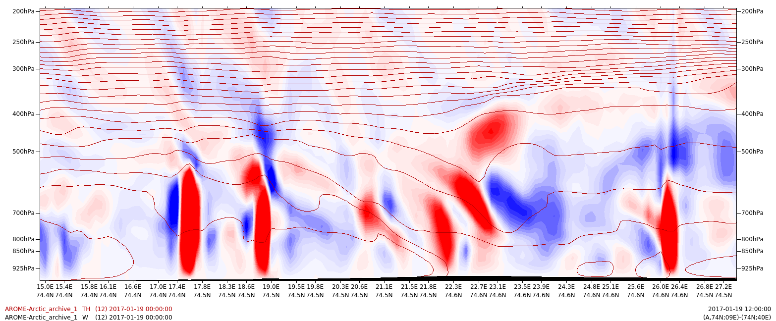
Figure 4.4: A plot along cross section B through the polar low showing θ (dark red) and ω (red/blue). The center of the polar low is located at 22 to 25 deg. E. Illustration: MET-Norway
Potential temperature and relative humidity
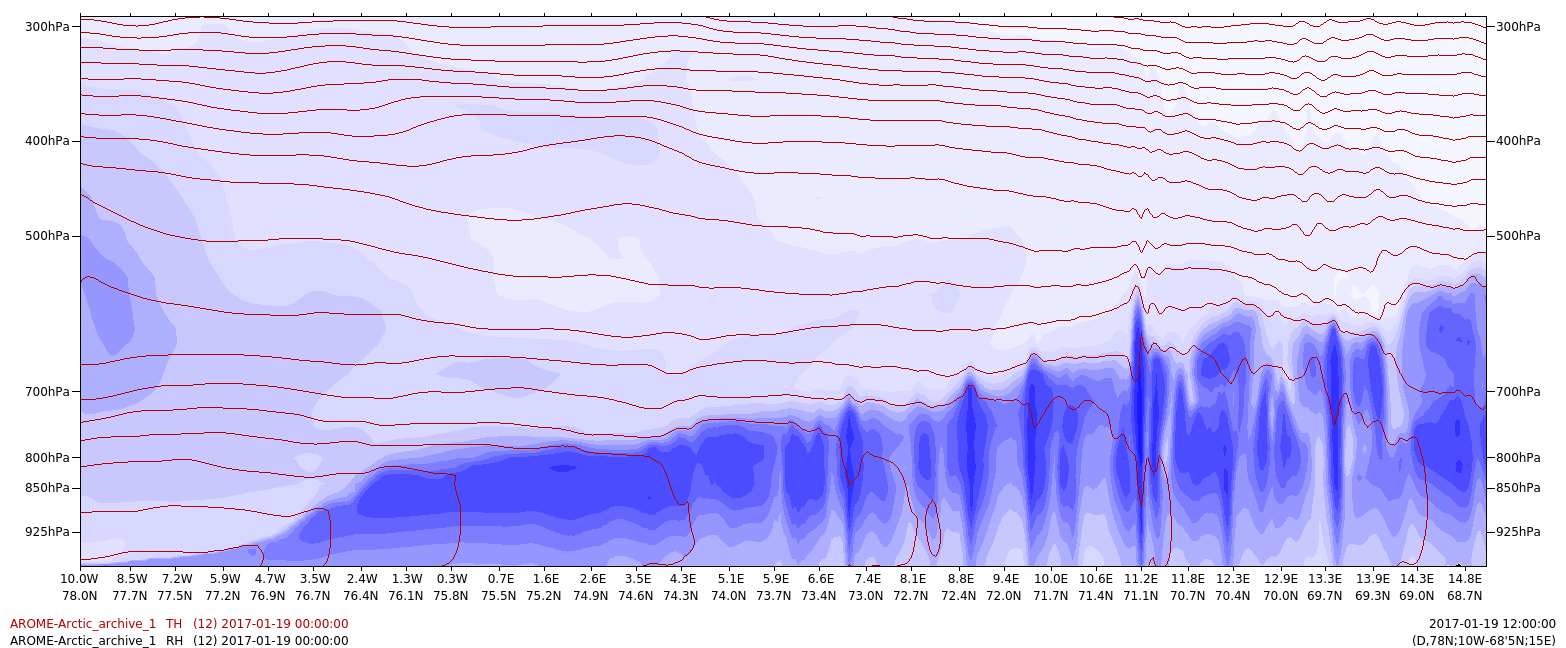
Figure 4.5: θ (dark red) and relative humidity (blue shading) along line A, along the cold air outbreak but west of the polar low: Illustration: MET-Norway
Figure 4.5 shows a cross section of θ and RH along line A. There is a strong flux of felt and latent heat from the sea surface, attending values of more than 500 W/m2 close to the ice.
The mixed layer increases in thickness as it is heated from below, and the cloud base increases from almost surface at the ice edge to typically 500 m at the Norwegian coast, and to 1000m if the cold air outbreak reaches the central North Sea. The vertical extent of the convective clouds is limited by the capping inversion until this is overcome by the heating from below.
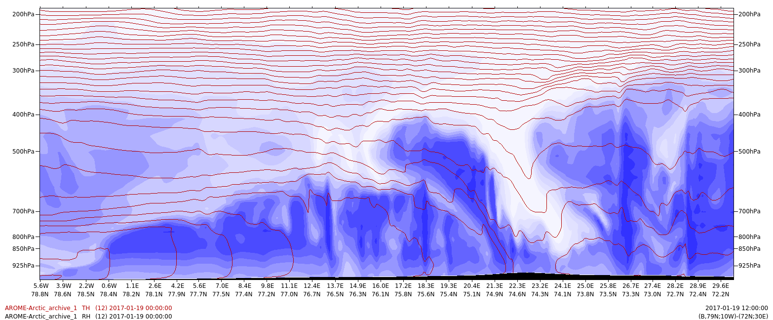
Figure 4.6: shows a similar plot along line C from the Greenland east ice through the polar low, located between 19E to 27E. Illustration: MET-Norway
The capping inversion extends southeastwards in this case to approximately 19E. Further downstream the inversion is broken down, and the air mass becomes unstable up til above 400 hPa. Here the moisture is transported upwards and outwards under the inversion at 400 hPa around the sides of the low center. The center itself can be seen as the dry and warm area from 22E to 25E. In this case it has a slightly backwards tilt, but in many cases the eye of the polar low is almost vertical.
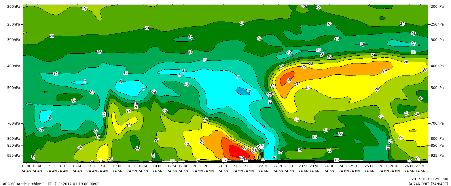
Figure 4.7: A closeup of the wind along cross section B, from west to east through the center. Illustration: MET-Norway
This low had reversed shear at low levels, which is typical for polar lows. This means that the wind from the thermal gradient is in the opposite direction of the wind from the pressure gradient, and thus the wind is strongest at low levels and decreases with height. In this case a low level jet of more than 40 m/s is seen west of the center. This jet is normally found around the western half of the low. Polar lows are normally embedded in a southerly moving air mass, and generally the strongest wind is found on the side of the low that has a component along the direction of the background large scale flow. There is a sharp gradient in the wind from the jet to the center of the low where the wind is almost calm, in this case at 22.5E, which is also very typical of the polar low.