Polar Low

Cloud Structure In Satellite Images

Appearance In Satellite Data

Polar Lows are small, but fairly intense maritime cyclones that form poleward of the polar front (Rasmussen and Turner, 2003). The horizontal scale of the polar low is approximately 150 to 600 kilometers, and sustained wind at 10 meter height is near or above gale force (>13,8 m/s). On average, maximum observed wind is at 22 m/s. Polar lows are a wintertime phenomenon that occurs mainly from October until April. Because of their northerly position, their small scale and their appearance in the dark winter season, AVHRR IR or day/night channel 3-4-5 images are the best way to detect Polar Lows. At latitudes lower than 68 degrees north, Meteosat IR are also useful for detecting such systems.

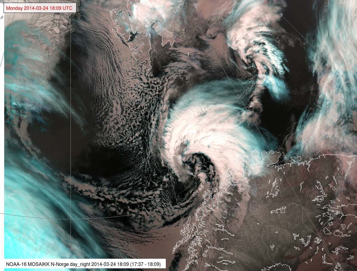
Figure 1.1: A mature Polar Low off the coast of Finnmark in Northern Norway from late March in 2014. This image is a combination of channels 3, 4 and 5, commonly known as the 'day/night combination. White is high and cold clouds. Grey is low/warm clouds. Black is sea. Blue/greenish is cirrus or high ice clouds. Illustration: MET-Norway/NOAA

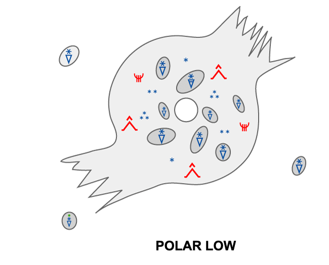
As can be seen from the various pictures in this section, the typical shape of the Polar Low is that of a non-symmetrical small cyclone around a dark and nearly cloud free eye. Normally there is an opening in the cloud mass south of the center. In the northern to eastern part there is a high and smooth cirrus shield, but in some cases with bands of convection is seen in this area. To the left of center is the tip of the cloud band, often with lower cloud top temperatures indicating that there is some descending motion here. This area is where the strongest winds are located around the low. Frequently also a wavelike feature can be seen at the western or northern edge of the cloud mass, indicating shear between the circulation around the low and an overlying jet.

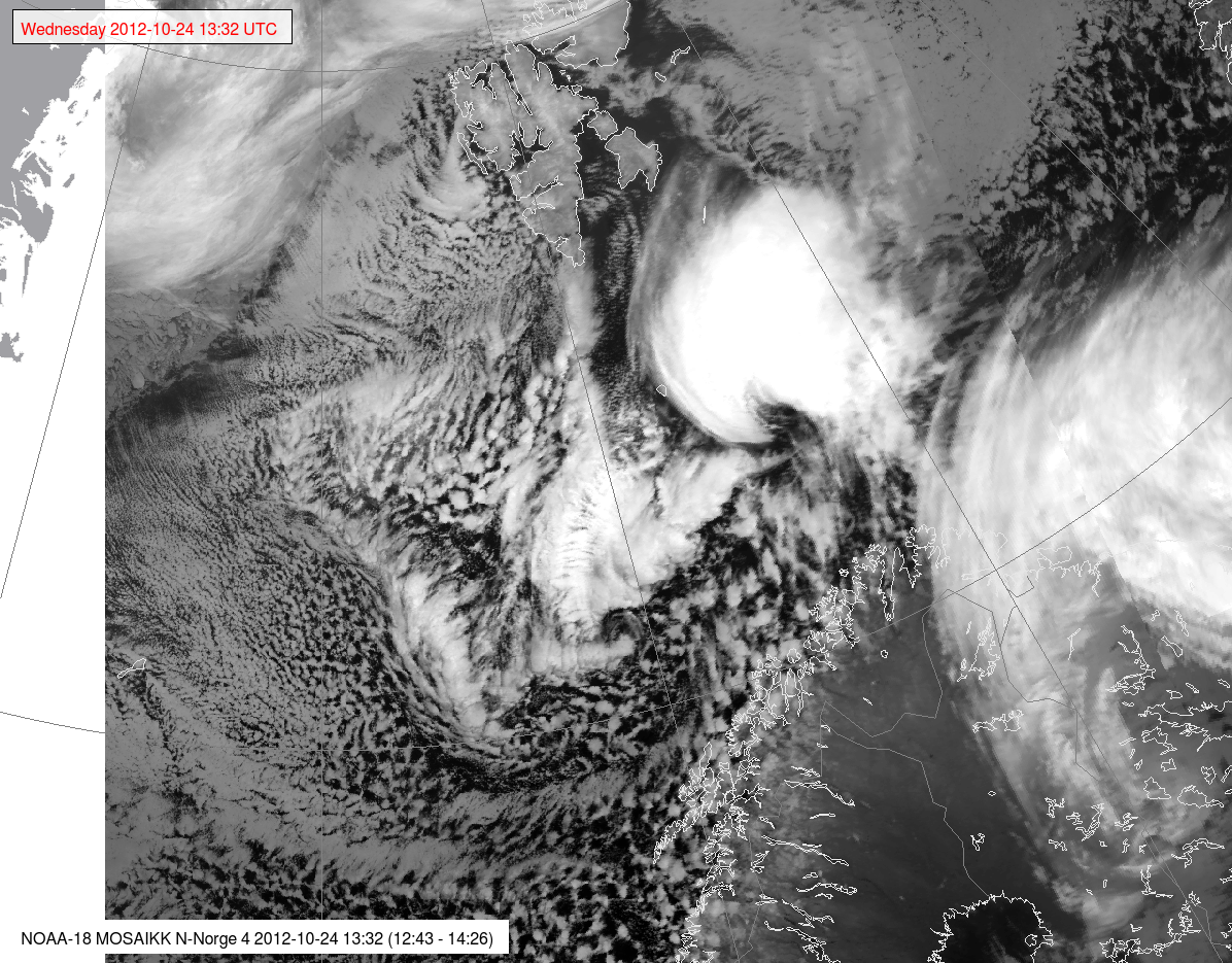
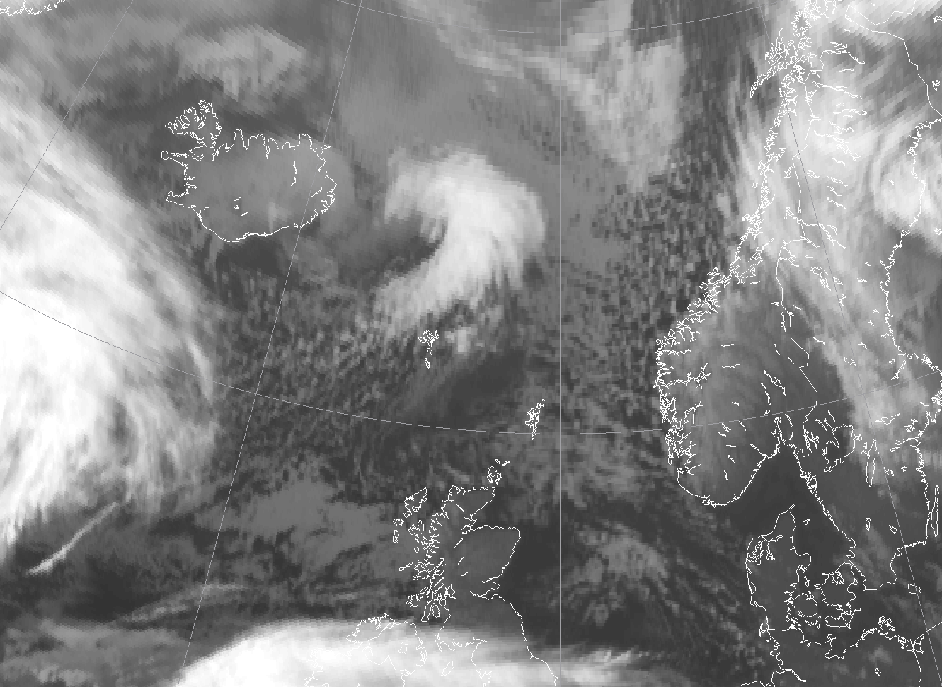
Figure 1.2: IR-image of a mature polar low southeast of Bear Island. To the southwest of this is a smaller low in its developing phase, and still further southwest is a north-south oriented trough where some cyclonic curvature and an emerging eye can be seen. Illustration: MET-Norway/NOAA

Polar lows is most common in the Norwegian Sea and the Barents sea, mainly east of the 0-meridian, and between 65 and 76 degrees north, but cases are known all the way south to the North Sea coast of continental Europe. Another area with high occurrence is to the south and east of the south tip of Greenland. These lows can usually be classified as lee lows or comma clouds in an easterly moving air mass, and do mainly affect the waters around the British Isles and the North Sea. The Japan Sea is known to be a prolific area for polar low formation. The Hudson Bay has some cases in the ice free autumn season, manly in October and November. There are also Polar Lows in the Antarctic, but since winds here are mainly zonal, cold air outbreaks from the ice is less persistent, and PL's here are generally weaker than those found in the Arctic.

Three different phases in the life cycle of a Polar Low can be distinguished: the initial/development phase, the mature phase and the decaying phase. It is also useful to consider the cold air outbreak since this is a necessary precursor for Polar Low formation.

The cold air outbreak

Polar lows are uniquely associated by cold air outbreaks (CAO) from the polar ice, and the CAO can be seen as a precursor to PL formation. Cold air outbreaks can easily be seen from satellite imagery. As the cold air flows out over open water, convection forms along lines oriented in the direction of the air flow in so called 'cloud streets'. These form a very intuitive impression of the flow in the mixed layer.

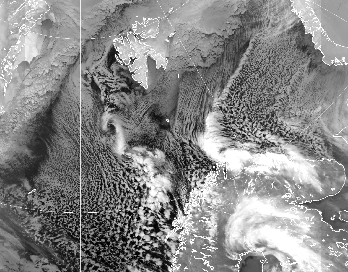
Figure 1.3: A cold air outbreak from March 2013. Cloud streets are clearly visible, as well as two convergence lines. The flow is generally in a southerly direction, and both convergence lines develop into very deep convection as they approach the Norwegian coast. illustration: MET-Norway/NOAA

Convergence lines forms where air masses meet, and these are prone to intensify into polar lows or other deep convection. In figure 1.3 a mature CAO is shown extending from Greenland till Novaya Zemlya. The wedge shape of Spitsbergen is particularly effective in modifying the flow to converge in the areas around Bear Island.

The developing phase

A developing Polar Low has the structure of a cyclonic curl that emerges from an otherwise more unorganized cloud mass, e.g. an old occlusion, a Cb-cluster or a convergence zone. Surrounding the emerging cyclone are cloud streets of shallow convective clouds with relatively low tops (darker grey in IR), typical for a cold air outbreak. The inner part of the curl shows sharp cloud edges while the outer part is often capped by cirrus cloud with fussy edges.

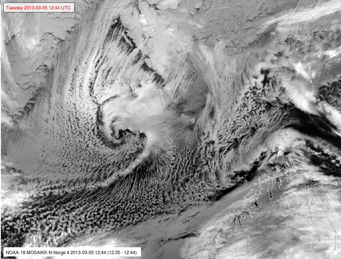
Figure 1.4: An Arctic front or convergence line extending westwards from Spitsbergen is curling up and starting to grow into a Polar Low. The eye and the cyclonic curvature is what distinguishes it from a trough or convergence line. Very white clouds west of Spitsbergen shows that this air mass is very cold and has potential for deep convection and Polar Lows. Illustration: MET-Norway/NOAA.

Mature stage

The cloud structure of a mature Polar Low is often a pronounced vortex with a (partly) cloud free and warm eye. The eye consists of relatively warm subsiding air at the center of the low, and it shows up dark or almost black in the IR image. Surrounding the eye is a continuous area of deep convection with strong vertical updraft and with heavy precipitation. This extend all the way up to the tropopause, which can be quite low in polar low situations, typically at 5 to 7 kilometers. Under the tropopause, the ascending air spreads out in a smooth cirrus shield that appears as bright white in the IR images. In some cases can be seen wavelike ripples extending out at the fringes of the cirrus shield. These indicate that there is an overlying jet and a wind shear at the top of the convective layer. Clouds at the 'tip' of the spiral tend to be less bright, indication tops at a lower level and that there are descending motion in this area.

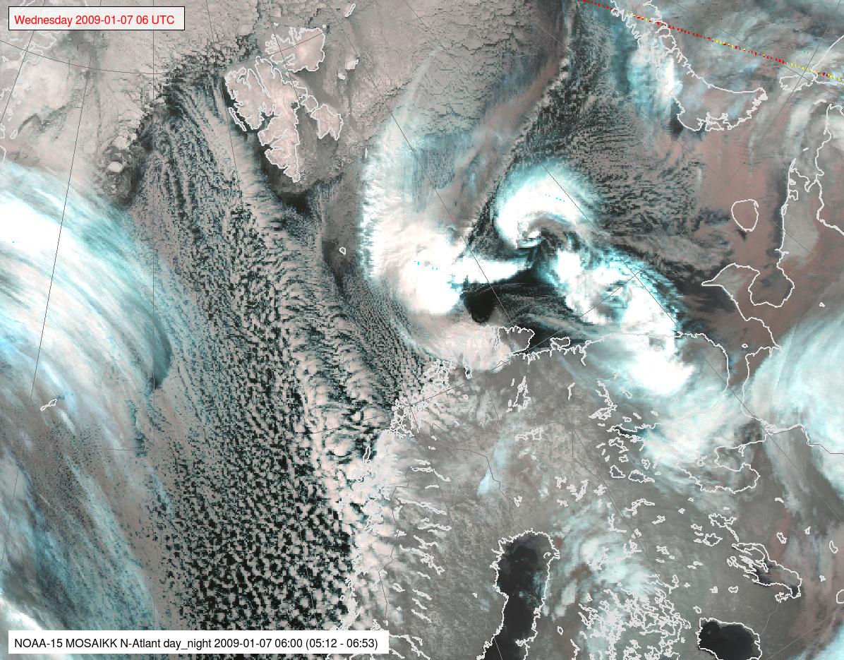
Figure 1.5: A mature polar low hitting the coast of Finnmark in January 2009. The eye can clearly be seen, as well as the smooth cirrus shield on top. Quite often polar lows appear in clusters of two or more, in this case there are two smaller eddies east of the main center. Illustration: MET-Norway/NOAA

Decaying phase

The most common reason for dissipation is that the low makes landfall. When the energy source from the warm sea is cut off and the low moves in over cold and dry land, it quickly loses its momentum.

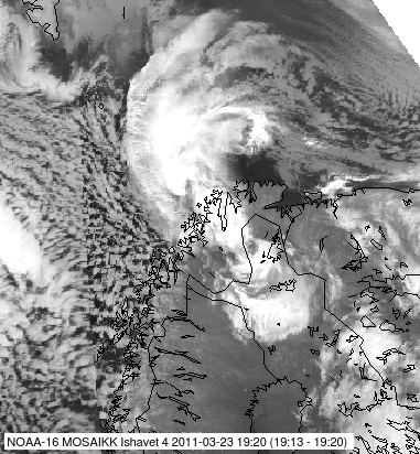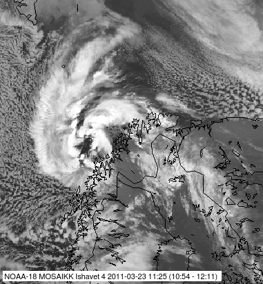
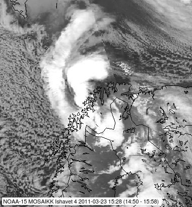
Figure 1.6: A Polar Low from march 2011 at different stages of landfall dissipation. To the left is at mature stage over open waters. Middle is just after landfall. The wind has subsided, but heavy precipitation is still present. On the right only high clouds remains. Although the cyclone can still be seen, the low has little impact on surface weather at this stage. Illustration: MET-Norway/NOAA

Negative vorticity advection is another effective way to weaken a low; the upper trough moves off and is replace by a ridge. In such cases the convection dissolves into more stratiform cloud types. An approaching warm front will also act to stabilize the air column, and will effectively stop a Polar Low in its development. From AVHRR images the low simply seem to vanish under the leading edge of the frontal clouds, and it soon loses its strength also at the surface.

Frequently a polar low dissipates while still over open water. Often the best sign of this kind of dissipation is that the cloud pattern becomes more disorganised. The cirrus is less visible or absent, and more is seen of the Cb cells or bands of convection at lower levels. These have a more chaotic flow under the cloud base, as opposed to the well organized inflow that exists at low levels around a mature polar low.

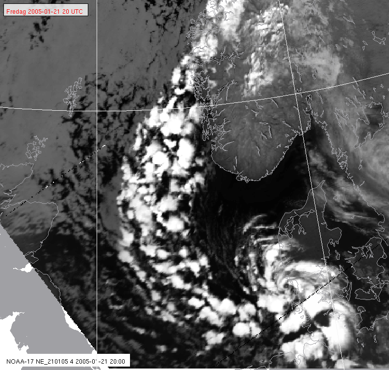Figure 1.7: A decaying polar low hitting the coast of Denmark in January 2005. The cirrus shield is gone, and individual Cb cells can clearly be seen. There is still some cyclonic curvature in the band of Cb's. This low will still give gale force winds and quite heavy precipitation. Illustration: MET-Norway/NOAA

Meso circulations and shallow polar lows

There are low pressure systems that have similarities to a polar low, but that are less intense and have less impact on the surface weather. Inspection of satellite imagery can give important information on the nature of these lows and help assess the depth of these lows.

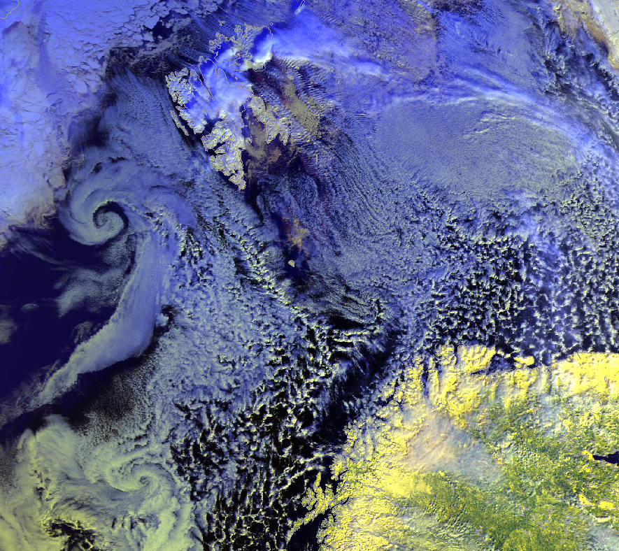
Figure 1.8: A meso circulation southwest of Spitsbergen on the 31st March 2014. Illustration: MET/NOAA

Illustration 1.8 shows a typical meso circulation southwest of Spitsbergen. The low brightness of the cloud and the fact that this is the same as that of the clouds surrounding it indicates that this low is not penetrating through the inversion above the Marine Mixed Layer (MML). Also, it has a smooth appearance of stratiform clouds at the top, but no cirrus. Hence this is a shallow low, often called a 'Meso Circulation', where the convection is confined to the mixed layer. Such lows usually have limited impact of one to two Beaufort on the surface wind.

In some cases very strong wavelike cloud patterns can be seen around the periphery of the cloud mass of the low, as shown in the example below. This indicates that there is a strong capping inversion and strong windshear above this, typically from an overlying jet. In the example shown, the flow in the MML was northeasterly, but above this there was a northwesterly jet. The ripples are waves in the shear zone between the to layers. Although it looks dramatic, this is usually a sign of a moderate vertical extent and moderate impact on the surface weather.

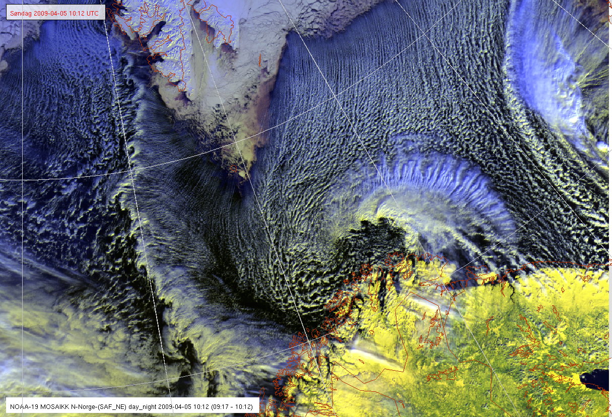
Figure 1.9: A shallow polar low north of the Finnmark coast, with unusually large wavelike cloud pattern around the center. Illustration: MET-Norway/NOAA

Appearance in geostationary Meteosat imagery

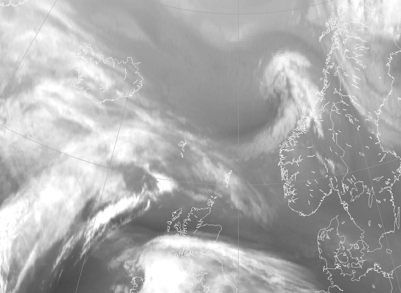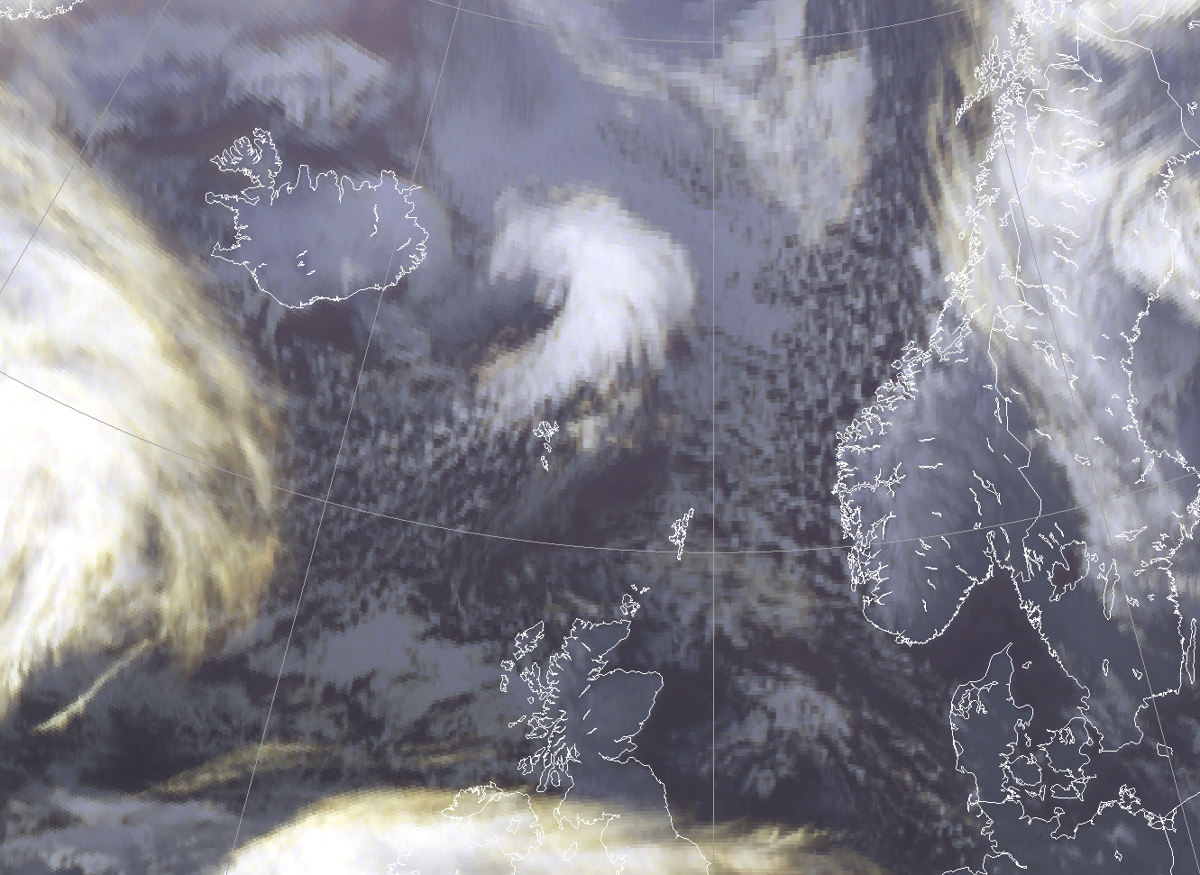
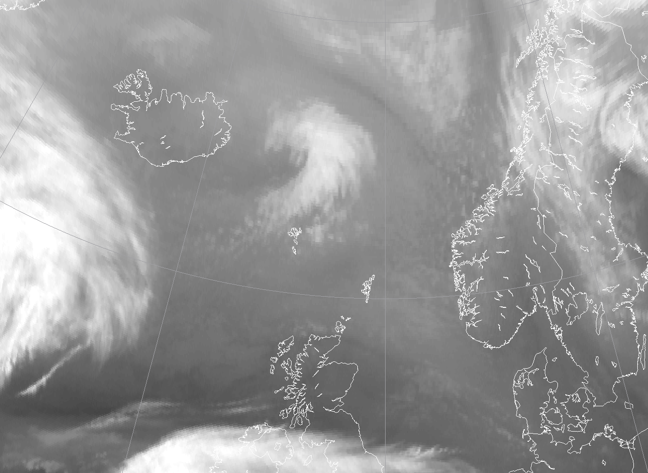
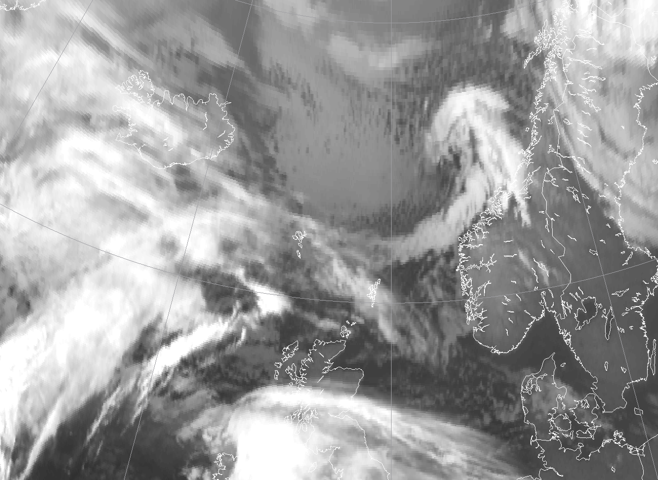
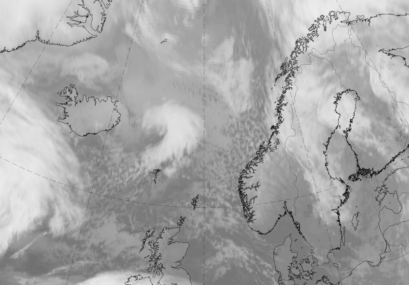
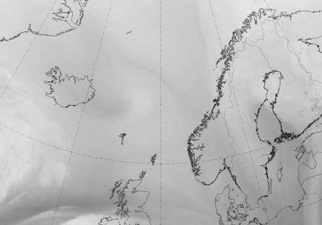
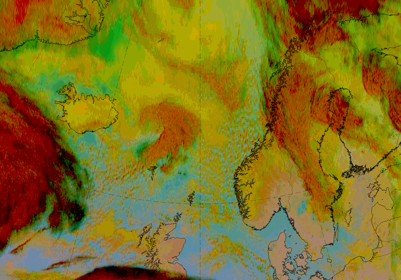
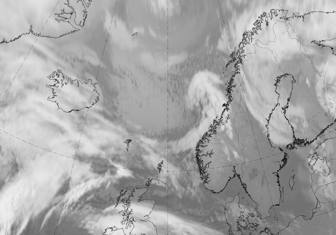
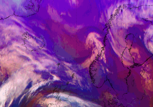
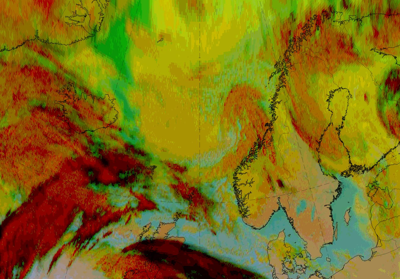
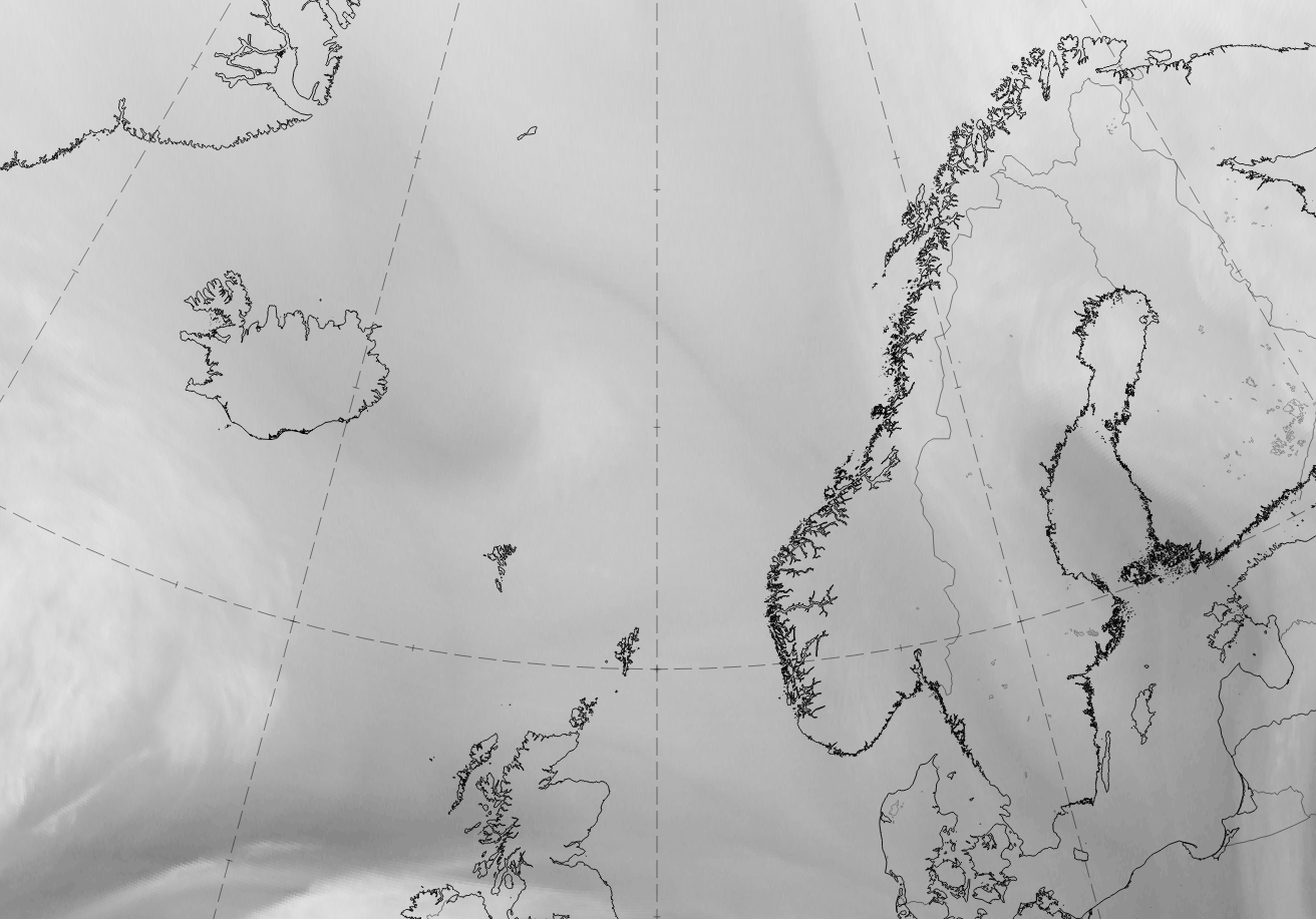
Figure 1.10: Meteosat images of a forming polar low east of Iceland on 4 December 2018

If the Polar Low is not too far to the north, it is possible to trace it with Meteosat images. In the first row above, a Comma shaped Polar Low is developing east of Iceland on the 4 December 2018. The left IR image shows the mature stage in IR channel 10,8, then the combination IR12.0, IR10.8 and IR3.9, and to the right the water vapour channel WV7.3. In the lower row can be seen the low at a later stage, just before landfall at the coast of Norway. From the dark areas in the WV channel can be seen that there are some tropopause folding associated with this low, indicating a frontal structure in the cloud bands around the center. Comma clouds in southwesterly flow is common in the central North Sea, often having an origin as a lee wave off the south tip of Greenland. These often have a stronger similarity to baroclinic synoptic low than the more convectively driven polar lows further north.

The case of 4 December 2018 can also be seen in the basic RGBs and compared among the basic channels and RGBs.

*Note: click on the image to access the image gallery (navigate using arrows on keyboard)

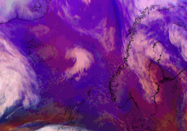
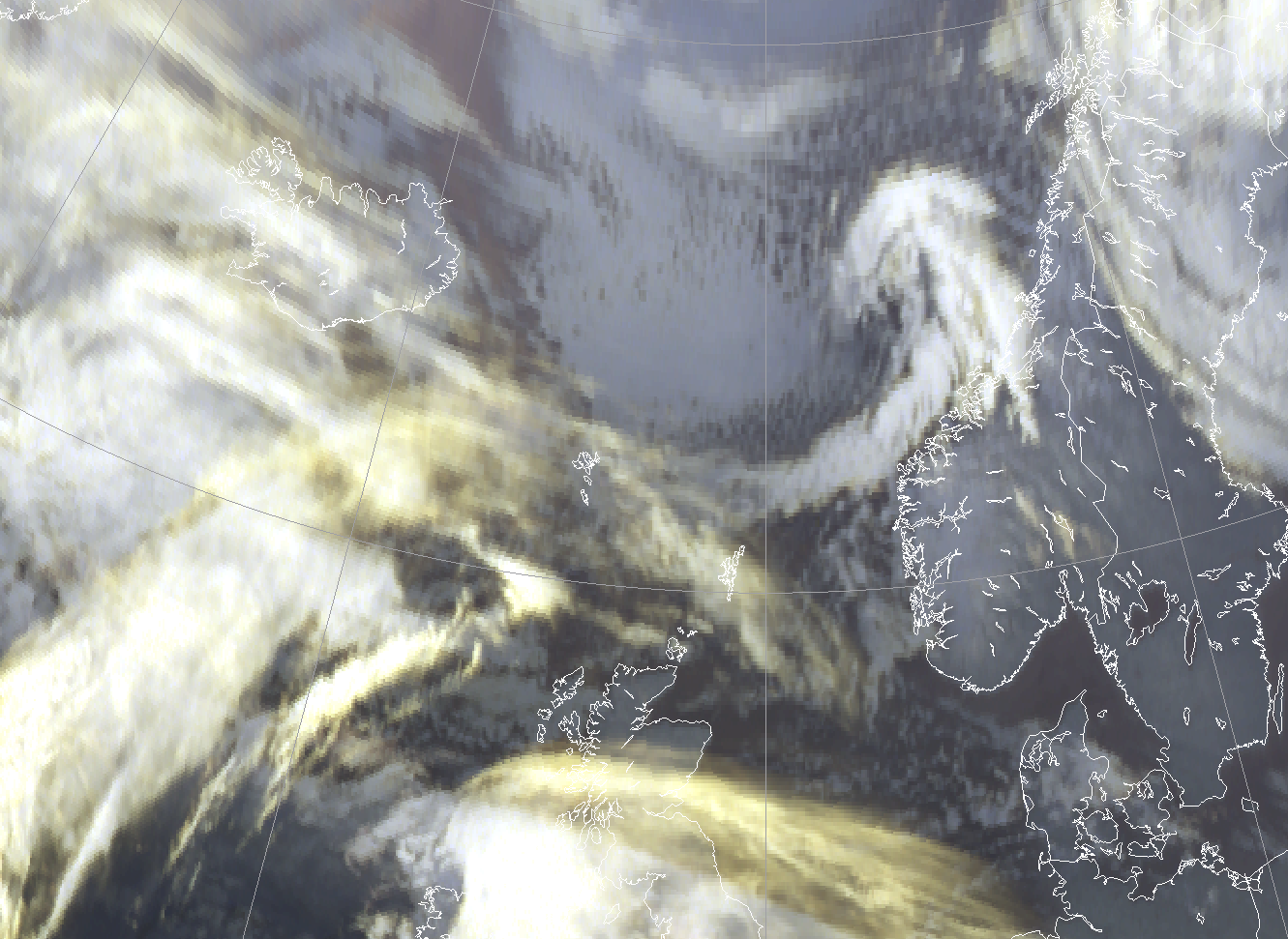
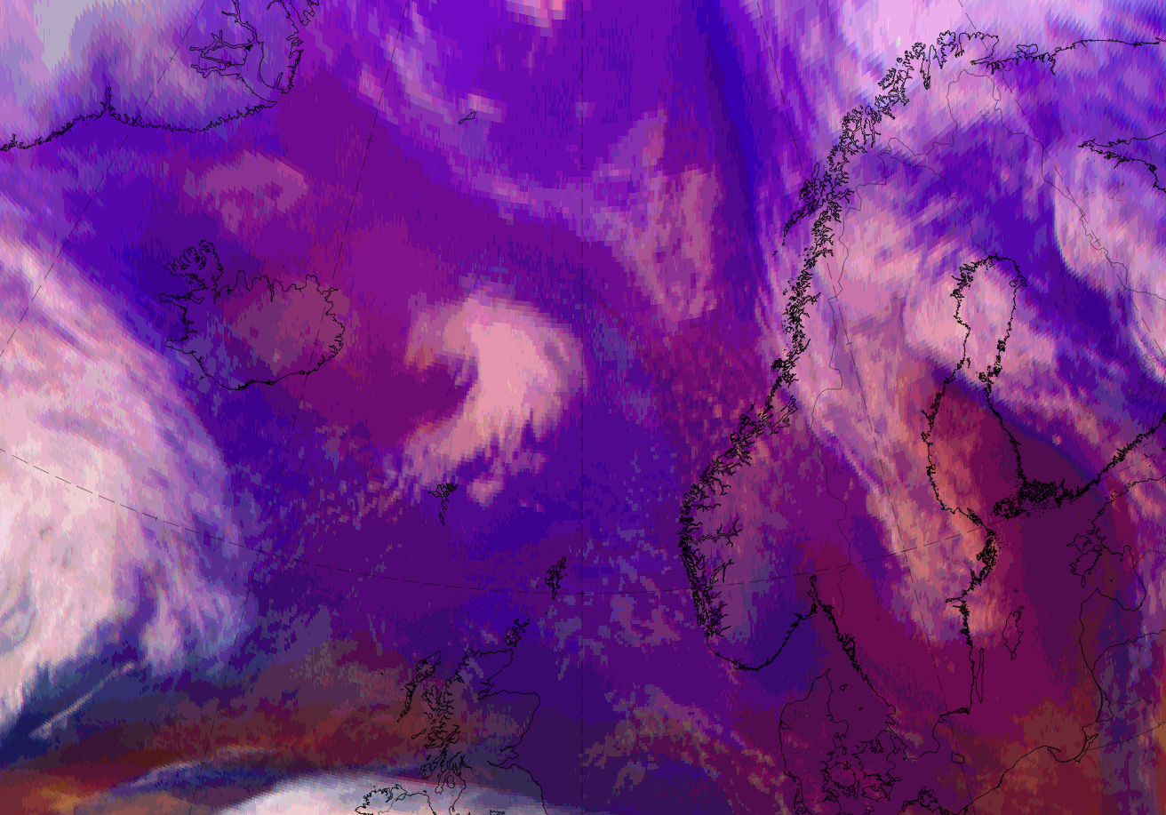
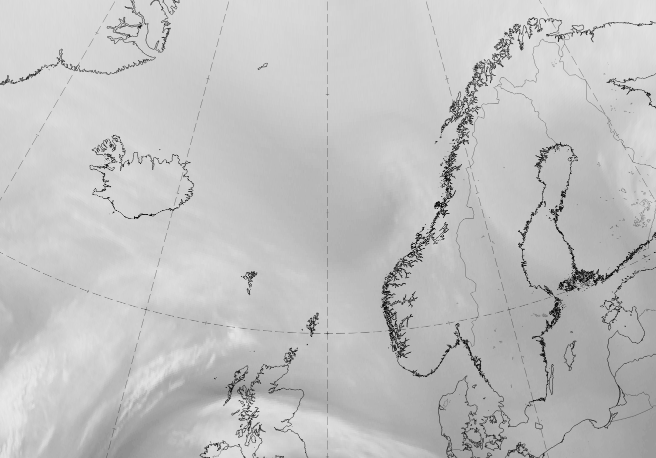
4 December 2018, 18UTC: 1st row: IR; 2nd row: WV (above) + Airmass RGB (below); 3rd row: Dust RGB + image gallery.
*Note: click on the image to access the image gallery (navigate using arrows on keyboard).

*Note: click on the image to access the image gallery (navigate using arrows on keyboard)

5 December 2018, 06UTC: 1st row: IR; 2nd row: WV (above) + Airmass RGB (below); 3rd row: Dust RGB + image gallery.
*Note: click on the image to access the image gallery (navigate using arrows on keyboard)

The two points of time representing the fully developed and the mature stage show very similar features in the basic channels and RGBs.

IR	Distinct white comma spiral; innermost part of the comma head is light grey, representing warmer temperatures.
HRV	No visible channel available in this geographical latitude and at this time of year and day.
WV	Cloud features are light grey; behind the polar low there is a dark grey area to the west. Northwest to the rearward edge of the comma spiral there is sinking stratospheric air.
Airmass RGB	Comma cloud embedded within dark blue colours representing the cold air behind the polar front. A dark red area behind the comma extends from the northwest to the rear edge of the comma spiral and represents the stratospheric, drier air. The comma cloud is overlaid by the dry air, hence the (usually white) clouds appear to have reddish colours.
Dust RGB	The comma feature is light red to brown, representing thick ice cloud but with lower cloud tops, as expected in thick comma features. Ochre colours around the comma cloud represent low to mid-level cloud, green colours represent mid-level cloud.

Other sources of satellite imagery of Polar Lows

As polar lows normally form over the vast sea areas at high latitudes, the are few synoptic observations available. However, there are several types of satellite instruments that measure wind at the sea surface based on the back-scattering of active radar. The back-scatter is affected by the capillary waves at the surface, which is directly dependent on wind speed (and direction). Such measurements are known to be heavily contaminated by rain, but less so by snow, and hence they are quite useful to study Polar Lows.

ASCAT

The ASCAT and previously the Quickscat is the currently main source of information of wind over sea, and when combined with ordinary IR satellite imagery, gives excellent information. As of 2018, the resolution is 12,5km. The ascat gives information on wind speed and direction. An artifact of the instrument design is that the wind direction have three possible solutions, and the best guess based on a model input from the ECMWF-HIRES is selected. In a Polar Low where there are very sharp gradients in speed and direction, the model guess is not always correct, so errors in direction is common, but this is of less importance since a correct guess of the direction can be made by comparing with an IR-satellite image or simply considering the known and quite predictable wind pattern around a Polar Low.

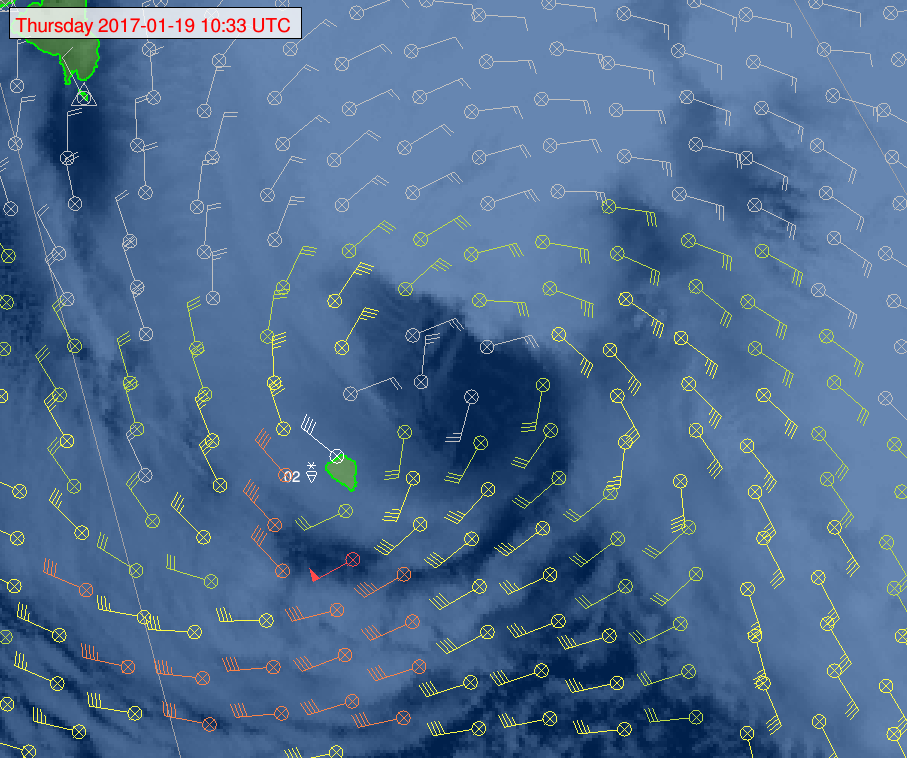
Figure 1.11: A close-up of ASCAT winds combined with an IR AVHRR satellite image with is made 50% opaque shows storm force winds southwest of the center of the low. Also the synoptic from Bear Island (white) is included in this composite. Illustration: MET-Norway/NOAA/Eumetsat

SAR

Syntetic aperture radar e.g. from the Sentinel 1 has a resolution of 5x20m and as such gives a very detailed impression of the wind pattern at the sea surface. Currently the images cover quite small areas (20x20 km), at intermittent intervals of 100 km along the path. In earlier years the regularity were such that these were not part of the operational basis of observations, but this has been improve with the launch of the Sentinel 1. The SAR images are most useful for studying the finer details, e.g. the shear zones associated with polar lows.

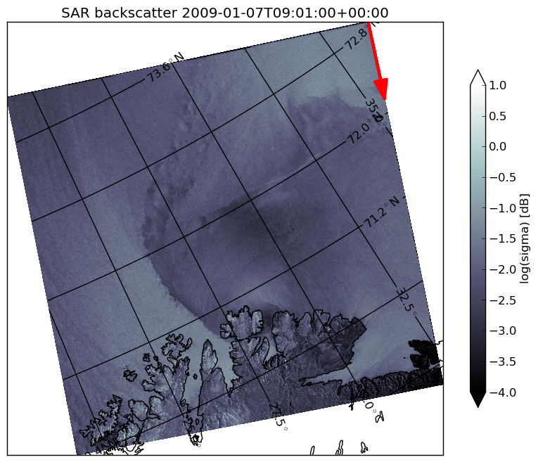
Figure 1.12: A rare SAR image capturing a polar low as it makes landfall at the coast of eastern Finnmark. Illustration: Furevik/MET-Norway

Bright colors in Figure 1.12 indicate strong winds. Dark is light winds. The shear zone between the western windy side and the eastern more quiet side is about 1 km wide, which explains why this is such a feared phenomenon in the coastal communities. The center of the low appears as dark, indicating that there are deceptively light winds here. The image also show that there is a smooth and focused flow around the center of a mature polar low, as opposed to the more disorganized flow in e.g. a cluster of Cb or a decaying polar low.

 

Meteorological Physical Background

Size of the Polar Low

Polar Lows develop within small baroclinic disturbances in a potentially unstable environment north of the polar front in the marine Arctic. The small scale of the Polar Low can be explained with the Rossby radius of deformation: R~N0H/f. In this equation, f is the coriolis parameter, N0 is the stability parameter, H is the scale height and R is the minimum scale of a system to be dynamically stable. The saturated-adiabatic lapse rate (small N0), the northern position (large f) and very cold air mass (small H), result in an R being significantly smaller in a Polar Low environment than in an environment of an extratropical cyclone.

Developing phase, necessary conditions

A polar low usually forms as a consequence of both baroclinic and static instability, the latter being almost unobstructed from low levels and up to above 500 hPa. In addition, also PVA at upper levels needs to be present. In the developing phase, the following elements are most common:

1. There needs to be a marine cold air outbreak (MCAO) at low levels within a marine mixed layer (MML). This layer is destabilized by supply of felt and latent heat from the ocean surface. The MML extends upwards to the inversion initially created by the cooling of the lower air mass as it passes over ice and snow covered surface. The top of this inversion is typically at 3 to 5 km height.
2. There needs to be a cold air mass above the MML, and an unstable stratification from the inversion layer at the top of the MML and up to at least 500 hPa. The rapid intensification of a Polar Low takes place when the MML is heated sufficiently so that the inversion layer above the MML is broken down and unobstructed static instability all the way up to above 500 hPa is achieved.
3. Positive vorticity advection (PVA) is supplied by an upper trough, most easily seen from the geopotential in 500 or 300 hPa. In the context of a polar low, there are usually quite low values of PVA, associated with a slow moving upper trough, but acting over a longer time period.
4. There needs to be an area of enhanced baroclinicity at low to middle levels that can, under influence of the upper trough and together with static instability, intensify into a Polar Low. The baroclinic zone can have different origins. Most commonly it is: 1) a remnant of an old occlusion, 2) a convergence zone, e.g. the one that often forms south of the tip of Spitsbergen in a northerly flow, or 3) at the fringes of a cold air outbreak, between the cold air in the north and warmer air to the south.

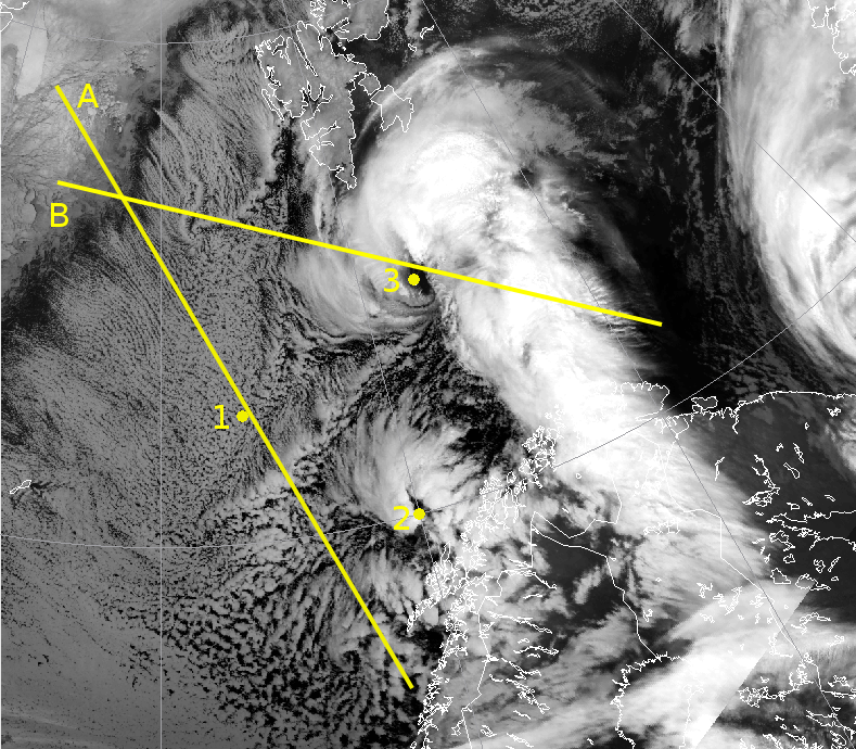
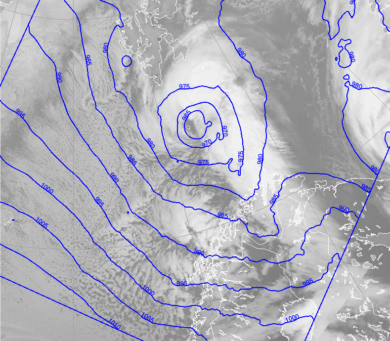
Figures 2.1a-d shows an example of a Polar Low and a cold air outbreak from 19th of January 2017 at 09Z, as seen with 0Z run from the Arome-Arctic 2,5km NWP model used at MET-Norway: In the upper left figure is the plain IR image, with cross sections and sounding points indicated. The main center is lying directly over Bear Island, and is moving in an easterly direction. The CAO is from the Fram strait west of Spitsbergen and the East Greenland ice cap. As the air leaves the ice, there is initially homogeneous convection with tops gradually increasing downstream. Approaching the Norwegian coast there is a cluster of enhanced convection and a small Polar Low. The upper right image shows the corresponding impression in the MSLP; a well defined closed low center, in this case almost symmetrical. The pressure pattern implies a strong northwesterly winds from the Greenland ice and an ongoing CAO.

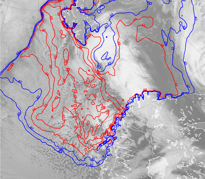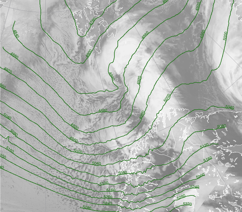
Figure 2.1: Four panes showing an example of parameters from the Polar Low from 19 January 2017 at 09 UTC. Illustration: MET/NOAA

The bottom left image shows a typical upper trough as seen in the Z500 geopotential, with a rather wide extent. Bottom right shows the SST-T500, which corresponds well in extent with the convective area. The main low is here situated in an area of steep gradient in the SST-T500, indicating that some baroclinic instability is present. The southern minor low is associated with an area of high values of SST-T500, so this low is mainly driven by deep static instability.

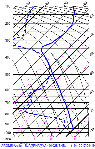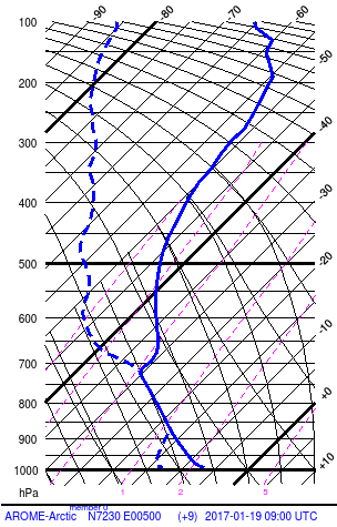
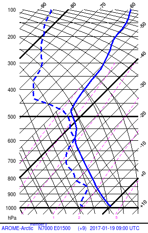
Figure 2.2: Figure 2.2: Soundings from point 1, 2 and 3 (left to right) in figure 2.1. Illustrations: Noer/MET

Figure 2.3 shows a cross section along line A. The marine mixed layer (MML) increases gradually in depth from the ice edge to the Norwegian coast where it attains a maximum height of 4000m (600 hPa), but the inversion on top of the MML is still not broken down. The left sounding in figure 2.2 is from point 1, midway along line A, and is typical for shallow convection with a strong inversion at the top, in this case at 3 km (700 hPa) height.

The sounding in point 2 is taken slightly northeast of line A, at an area with more deep convection. The main inversion here is at 6 km (500 hPa), consistent with the small polar low forming here. A lesser inversion at 600 hPa is at the same level as the top height of the MML seen at the southeastern end of line A. As can be seen from the cloud mass of the satellite image in figure 2.1a, this slight inversion is sufficient to stop the convection from reaching higher.

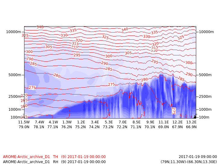
Figure 2.3: Cross section A across a CAO with moderate vertical extent. Red lines are potential temperature. Blue shading are relative humidity. Illustration: Noer/MET

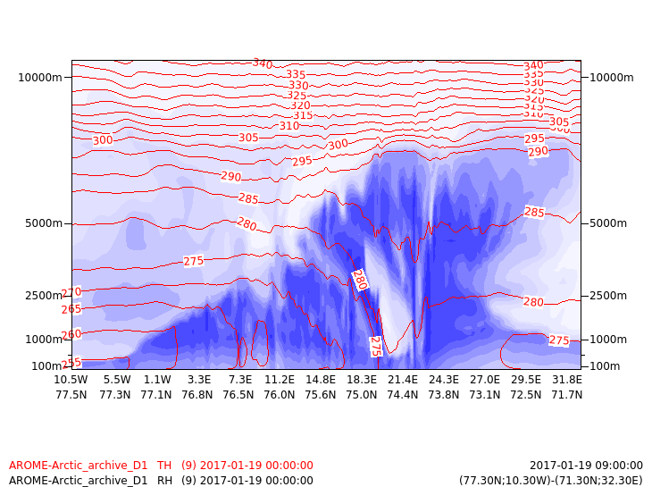
Figure 2.4: Cross section B across a polar low. Red lines are potential temperature. Blue shading are relative humidity. Illustration: Noer/MET

Figure 2.4 shows the cross section B through the polar low. The inversion is broken down around the center (east of 14E), and the moisture and clouds are transported up by convection to the tropopause at 7 km (400 hPa) height. The sounding at point 3 is at the center of the main Polar Low. The air column is unstable up to the tropopause at 400 hPa, and typically polar lows form in air masses where the tropopause is between 500 and 400 hPa. Comparing to the sounding at point 2, we see that the air mass above 500 hPa is colder at point 3, - there is an upper cold core present.

Synoptic situation, reversed or direct shear

Polar Lows often form in a northerly flow behind a major synoptic low, with the low center to the south or east but the cold air to the north or west of the center. In such cases the thermal wind is in the opposite direction of the pressure gradient wind, and the wind will decrease and shift direction with height. This condition is called reversed shear, and is most common with polar lows. In this condition the upper trough is positioned above or ahead of the surface low, as opposed to the 'normal' direct shear case where the upper trough is trailing the surface low. Another feature often seen in reversed shear cases is that the reduction in wind speed in the vertical tends to be concentrated in a shear zone around the 850 to 700 hPa level. The steering level of the polar low is then found at the top of the bottom level, just below the shear zone.

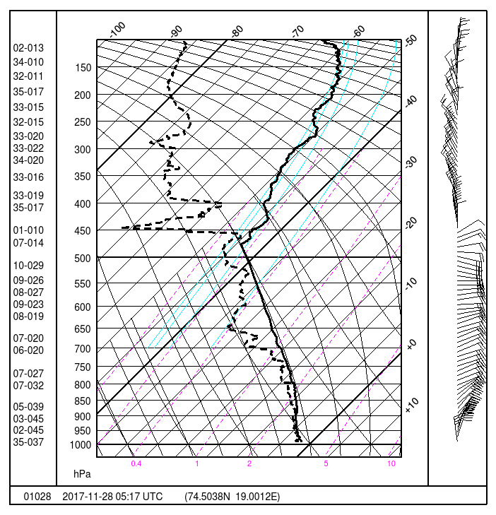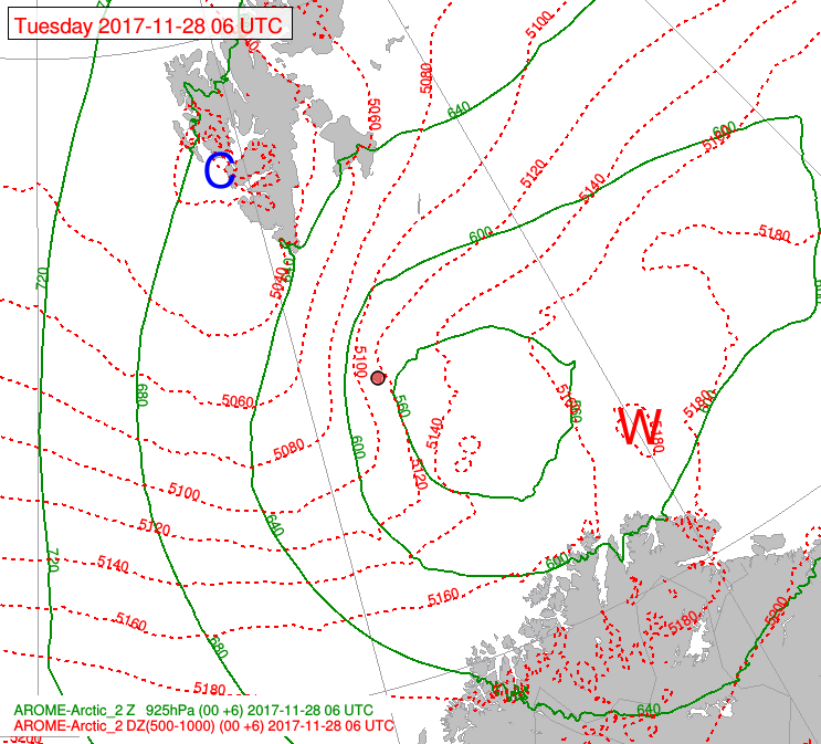
Figure 2.5: Reversed shear seen in a polar low from 17th November 2017.

Left image shows the geopotential in 925 hPa (green) and 1000 - 500 hPa thickness (red). In this case, the strongest gradients is in the area near Bear Island (red dot). The gradient in the thickness is in the opposite direction of the pressure gradient, hence the thermal wind acts to decrease wind with height. The right image shows the corresponding sounding from Bear Island. Wind direction and speed (knots) is given by the numbers on the far left in the sounding. In this case, the strongest wind is found at 900 to 950 hPa.

Spatial distribution of Polar lows

The amount of static instability in the MML is closely coupled to the supply of latent and felt heat from the sea surface, which in turn is dependent on the difference in the temperature of the air close to the sea surface and the sea surface itself. This is largest close to the ice edge, where the difference can be of more than 40°C, but of more importance is the difference further downstream as the cold air is advected over the warmer waters of the North Atlantic current. Especially where the air mass is advected across areas of steep gradients in the sea surface temperature (SST), e.g. at the edges of the various branches of the North Atlantic current, the airmass is prone to develop deep convection and polar lows. As can be seen from illustration 2.6, the polar lows mainly develop over the warmer areas of the North Atlantic.

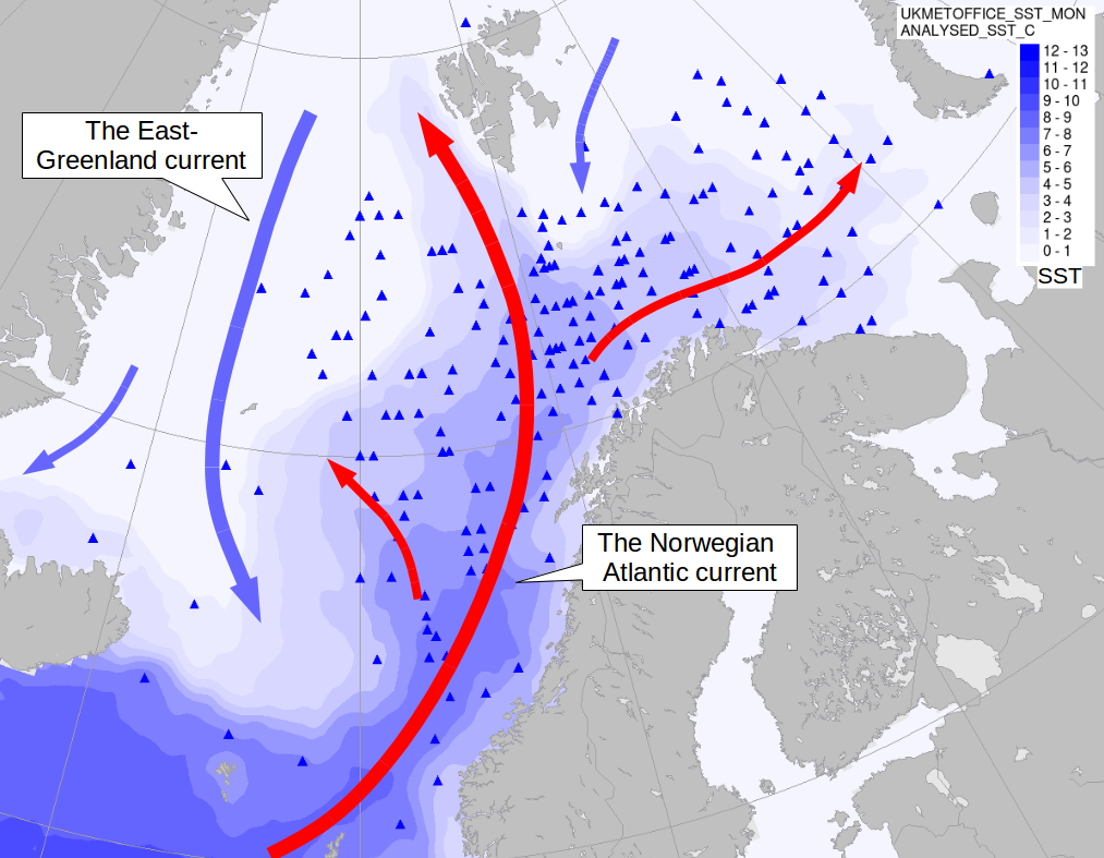
Figure 2.6: The genesis areas of polar lows from 2000 till 2017 plotted as triangles. Blue shading is monthly mean sea surface temperature in February (UK MetOffice). Also shown are the main ocean currents in the North Atlantic, showing the sourced of warm and cold water in the area. Illustration: Noer/MET

There is a slightly higher concentration in the area south of Bear Island. This is probably because this area receives CAO from both sides of Spitsbergen, as well as being subjected to convergence and enhanced convection off the south tip of Spitsbergen in northerly flow. There are less Polar Lows in the eastern part of the Barents sea because the SST and also gradients in SST are less in this area.

Because of the significance of the SST, to identify the cold cores that favor growth of polar lows it is more useful to consider the difference between SST and the temperature at 500 hPa. In earlier years when the location of the cold cores was uncertain, it was common to consider the max value of this difference, and a threshold of 44°C was used to indicate an area prone to PL development. In recent years, and especially when using the SST - T500 difference e.g. for automated tracking, the difference is taken in the same gridpoint. In such cases a lower value must be used, and 40°C is now considered to be the most appropriate.

This is also physically consistent with the fact that most polar lows develop as a result of a mix of static and baroclinic instability, and a common source of the latter is at the edges of the cold air outbreaks, between the cold and warm air masses, but where the temperature at 500 hPa is not as low as at the center of the cold core.

 

Key parameters

MSLP

The polar low is usually seen as a closed low of some 5 to 20 hPa lower center pressure than the surroundings. In some cases, if the large scale gradient is strong, the low may only be an open trough in the MSLP. The cold air outbreak is also best seen in the MSLP, as it gives information on the origin and the flow of the air mass. For the air mass to be sufficiently cooled, it needs to spend some time over cold surface, hence a rather long trajectory above the cold surface is needed.

T500 and sea surface temperature (SST)

The deep convection associated with a polar low is to a large extent fuelled by the heat absorbed from the underlying sea surface, which is directly dependent on difference between the air temperature at the surface and the SST and maintained at a high level where the air is advected over areas with a steep positive gradient in the SST. Polar lows tend to form when the static instability reaches above 500 hPa, i.e in areas with relatively low values of T500. The difference between the SST and the T500 has proven to be a crude but most effective indicator for deep static instability over sea surface, and corresponds well with areas with either polar lows or deep convection. When taken vertically within a gridpoint, 40°C is a good threshold value for the triggering of Polar Low development. Historically, when the forecasted location of the cold cores were less precise, the maximum value within the cold air outbreak as a whole was used, and a value of 43 to 44°C is frequently referred to as a threshold value. Studies at MET-Norway have shown that polar lows form in about 25% of the times when this threshold is exceeded.

Z500 and positive relative vorticity advection (PVA)

An upper trough, often seen in the Z500 is often superimposed over the area of an initial Polar Low. In direct shear situations the trough is slightly behind the developing low. In a reversed shear case the upper low is slightly ahead. Statistical analysis shows the highest value of PVA normally occurs in the developing phase and gradually decreases in the following phases. Finally in the decaying phase the value is almost zero or may even be negative. Generally, deep convection tends to develop over several hours or days as it absorbs heat from the underlying rather cool surface. It is therefore more efficient for polar low formation with a shallow upper trough that is slow moving and has low values of PVA than a fast moving trough with high PVA. The latter case only acts over a brief time, and will therefore only give a marginal enhancement of the instability in the air column.

10m wind

A part of the definition of polar lows is a requirement of 10m wind of 'near gale' Beaufort 7 (> 13,8 m/s) or higher. This is a weak criterion since many similar phenomena give higher winds than this, so near gale force winds does not necessarily make a polar low. Nevertheless the 10m wind is an important aspect of the assessment of polar lows. The strongest winds are normally to be found at the position where the relative motion of the polar low is in the same direction as the actual wind, in other words on the western side of the low.

Cloudiness or 1h precipitation

The convection in a polar low is oriented as cloud bands, spiralling out from the center in a typical cyclone shape, seen in both satellite imagery and radar. The precipitation produced by the convection shows up similarly and gives an easily recognizable pattern in prognostic fields for e.g. 1hr precipitation.

Equivalent potential temperature θ_e

In most cases a Polar Low develops on a secondary shallow baroclinic zone in a marine cold air outbreak. This zone can be best visualised using the equivalent potential temperature θ_e contours at 850 hPa, showing the fronts and the gradients between warm and humid or cold and dry air masses.

Vertical Motion (Omega) 850 hPa

Because of unstable conditions and upper level forcing mechanisms, vigorous ascending motion could develop. As a result of a low tropopause, the ascending motion is present in a relatively shallow layer, making omega at 850 hPa more indicative than omega at 500 hPa.

During the development phase the enhanced cloud band is characterized by a negative omega with a relative minimum at the position of the developing Polar Low. This minimum expands and finally, in the mature stage, a cut-off minimum is present surrounded by a band of descending air with positive omega values.

Other indexes

The K-index is mostly used for summer convection, but can also be used for winter conditions, but then with slightly lower values, typically 15 to 20.

The Showalter Index (SI) and the Lifted Index (LI) take the difference between T500 and the parcel temperature at 850 and 925 hPa respectively. The Total-Totals (TTI) is similar to the SI, but considers also moisture at 850 hPa: TTI = (T850-T500)+(Td850-T500). However none of these consider the important aspect of transfer of heat from the sea surface as indicated by the SST, and are generally less used than the SST-T500 described above in the context of polar lows.

The Boyden index is given by BI = DZ(1000-700) + Td850 - 200, where the first part is the thickness below 700 hPa and the last part is a scaling to give the BI values between 90 and 100. The Boyden index is useful for considering convection, but it gives no information about conditions above 700 hPa. Hence it tends to give a rather flat field in areas with deep convection where the tops are typically well above this level.

 

Appearance in cross sections

The structure of a polar low can be further studied by looking at prognostic cross sections. For comparison we consider here cross sections along line A, typical for a well mixed marine Mixed Layer (MML) and along lines B and C, across the center of the polar low. Here fields from the Norwegian Arome-Arctic 2.5km model is shown, with a forecast length of 12 hrs.

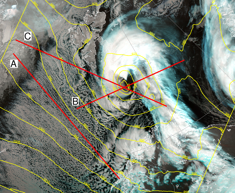
Figure 4.1: Cross sections (red lines) from the 19th January 2017, 12 utc. Yellow lines are a 12 hr. prognosis for MSLP, indicating a center at 74.5N 22.5E. Illustration: MET-Norway

Vorticity advection

One of the main dynamical mechanisms in the initial or developing phase is Positive Vorticity Advection (PVA) caused by a moving upper level through. To trigger a Polar Low, a PVA maximum has to be superimposed upon the baroclinic zone.

Potential vorticity

Potential Vorticity (PV) is an important parameter in the development phase of a Polar Low. In this stage an upper level PV maximum is normally just upstream of a Polar Low.

This PV maximum is situated at mid levels of the troposphere but has transferred down from the stratosphere. A PV maximum can also be found in the gradient zone of the very stable layer near the surface over or near icefields.

Vertical Motion

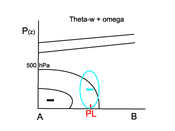
Figure 4.2: Vertical Motion (omega)

In figure 4.3 and 4.4 a stable layer is seen as horizontal isolines for the potential temperature (θ). Vertical orientation in the isolines for θ indicates a well mixed layer and a statically unstable air mass. In a cold air outbreak there is a strong inversion above the marine mixed layer. Figure 4.3 shows a cross section along line A west of the polar low. Here there is a homogenous layer of shallow convection which extends upwards to the inversion. Smaller areas of negative ω associated with individual convection cells can be seen adjacent to areas of positive ω, in the dry sinking air outside the convection cells. The absolute values of ω are of more than -3 hPa/sek, but the maxima are confined to small areas. Cumulus Congestus (often called towering Cumulus) usually have a horizontal extent of a few kilometers, but with sharp gradients between areas of ascending and descending air. For aviation, turbulence associated with TCu's are described as moderate.

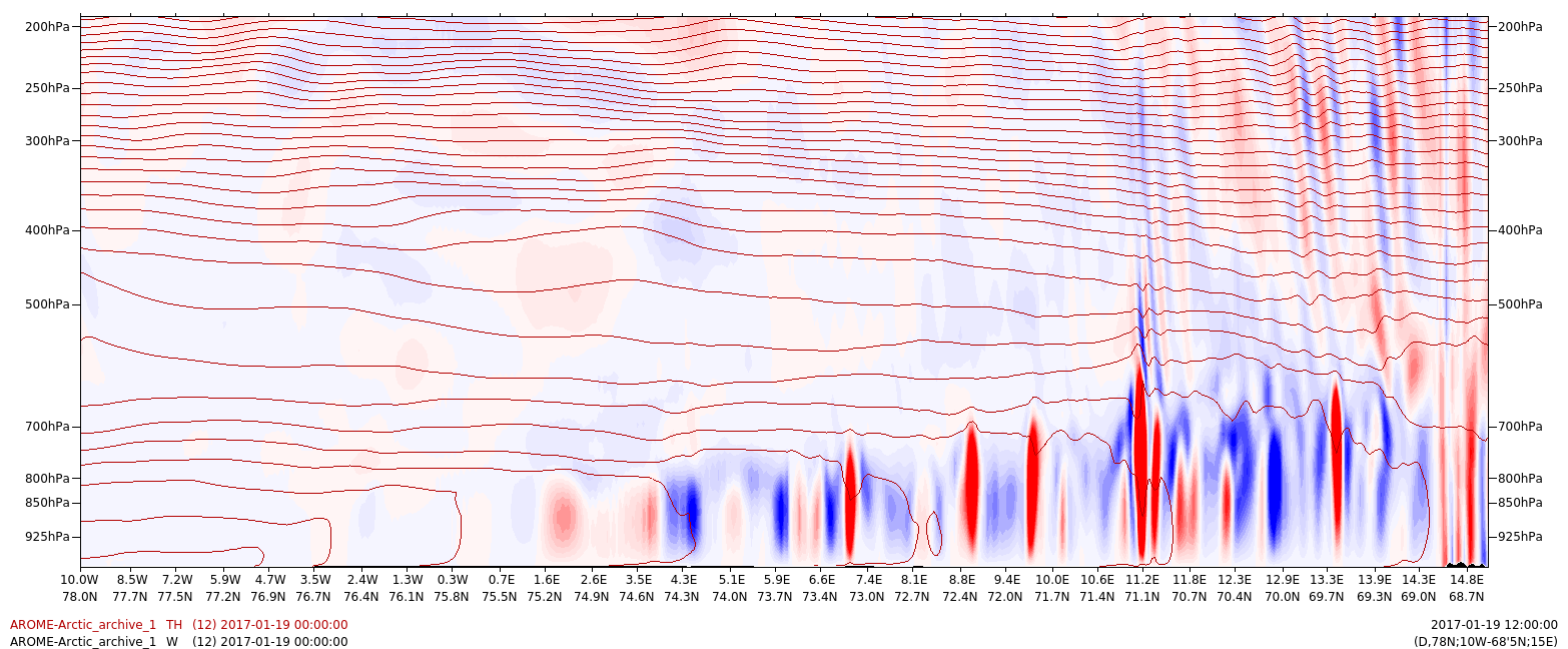
Figure 4.3: Shows potential temperature (dark red lines) and vertical speed (blue/red shading for +/- ω) along line A through the cold air outbreak to the west of the polar low. Illustration: MET-Norway

If the inversion above the MML is broken down, deeper convection can take place, and polar lows may form. A polar low will manifest itself as larger areas of ascending air and negative ω. The absolute values are similar to what can be found in more shallow convection, but the horizontal and vertical extent is larger. The negative ω is associated with the deep convection around the center of the low, in figure 4.4 seen as bands at 22 to 23 degree E reaching up to above 400 hPa. A polar low also has an eye of dry and warm descending air at the center, as can be seen in figure 4.4 as the area of positive ω at 23 to 24 degree E. Often lower (darker in the IR) cloud masses can be seen at the southwest of the center, at the tip of the cloud band, indicating descending air in this area.

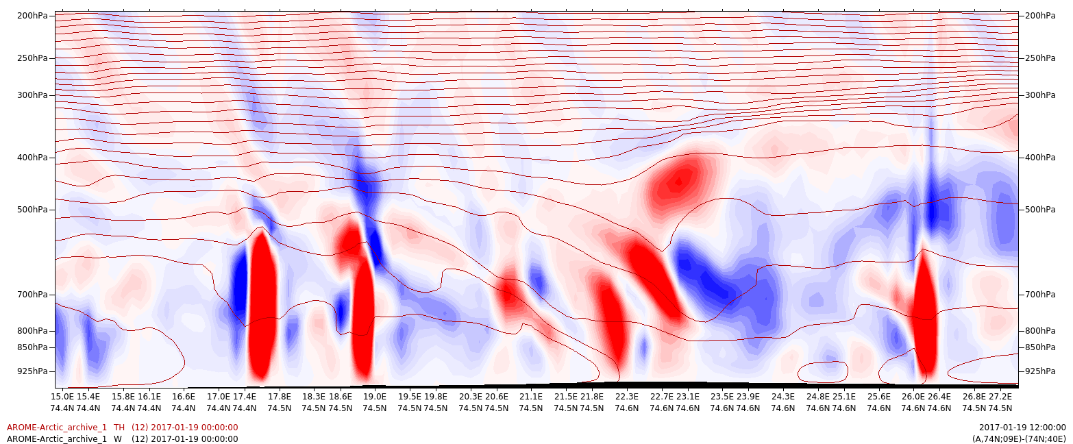
Figure 4.4: A plot along cross section B through the polar low showing θ (dark red) and ω (red/blue). The center of the polar low is located at 22 to 25 deg. E. Illustration: MET-Norway

Potential temperature and relative humidity

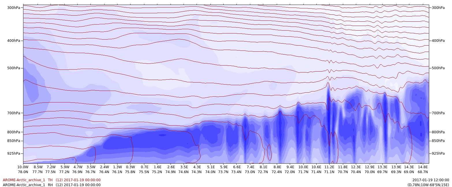
Figure 4.5: θ (dark red) and relative humidity (blue shading) along line A, along the cold air outbreak but west of the polar low: Illustration: MET-Norway

Figure 4.5 shows a cross section of θ and RH along line A. There is a strong flux of felt and latent heat from the sea surface, attending values of more than 500 W/m2 close to the ice.

The mixed layer increases in thickness as it is heated from below, and the cloud base increases from almost surface at the ice edge to typically 500 m at the Norwegian coast, and to 1000m if the cold air outbreak reaches the central North Sea. The vertical extent of the convective clouds is limited by the capping inversion until this is overcome by the heating from below.

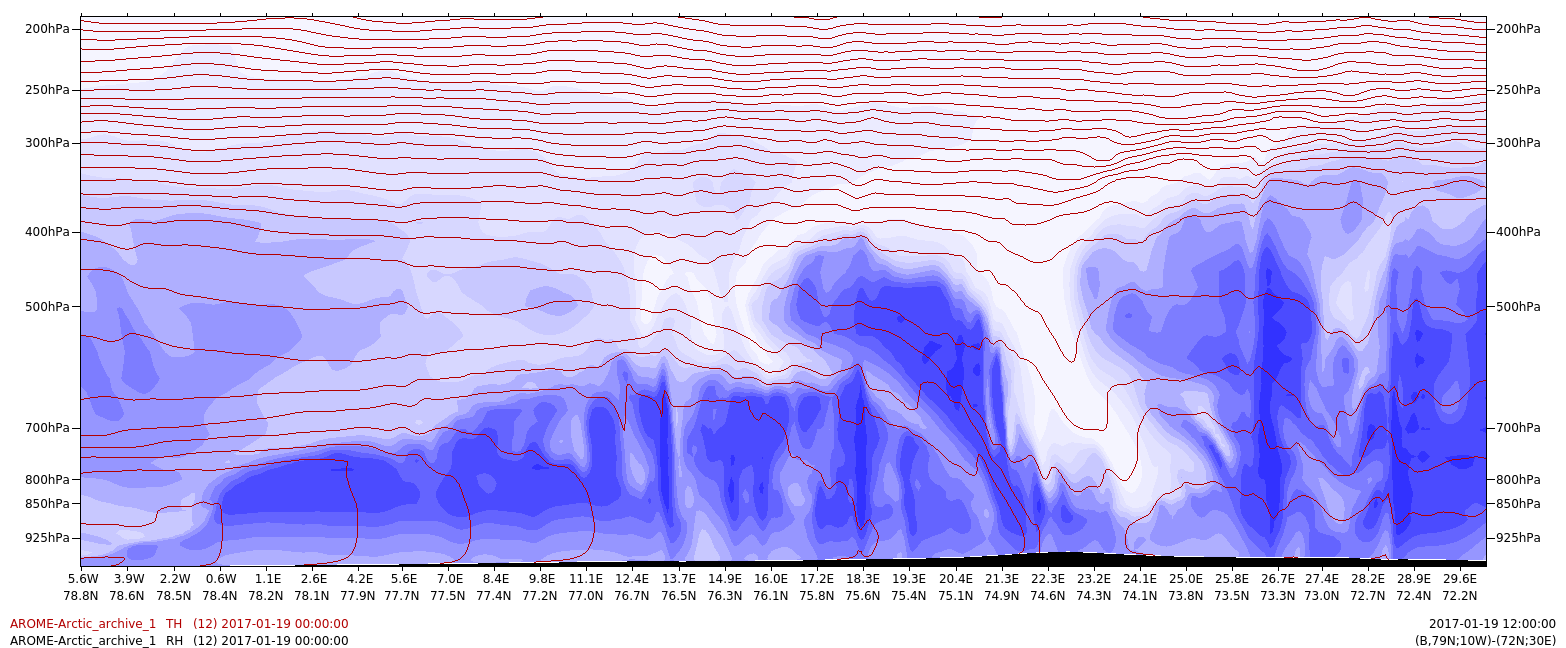
Figure 4.6: shows a similar plot along line C from the Greenland east ice through the polar low, located between 19E to 27E. Illustration: MET-Norway

The capping inversion extends southeastwards in this case to approximately 19E. Further downstream the inversion is broken down, and the air mass becomes unstable up til above 400 hPa. Here the moisture is transported upwards and outwards under the inversion at 400 hPa around the sides of the low center. The center itself can be seen as the dry and warm area from 22E to 25E. In this case it has a slightly backwards tilt, but in many cases the eye of the polar low is almost vertical.

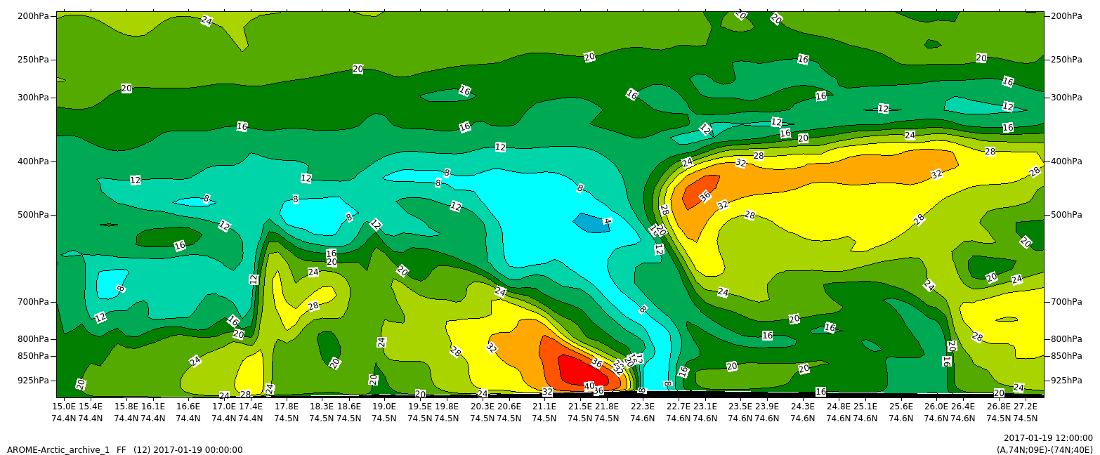
Figure 4.7: A closeup of the wind along cross section B, from west to east through the center. Illustration: MET-Norway

This low had reversed shear at low levels, which is typical for polar lows. This means that the wind from the thermal gradient is in the opposite direction of the wind from the pressure gradient, and thus the wind is strongest at low levels and decreases with height. In this case a low level jet of more than 40 m/s is seen west of the center. This jet is normally found around the western half of the low. Polar lows are normally embedded in a southerly moving air mass, and generally the strongest wind is found on the side of the low that has a component along the direction of the background large scale flow. There is a sharp gradient in the wind from the jet to the center of the low where the wind is almost calm, in this case at 22.5E, which is also very typical of the polar low.

 

Weather Events

A polar low is normally embedded in a southerly moving air mass, and generally the wind is strongest on the western half of the low where the circulation of the low has the same direction as the ambient large scale wind. The most dangerous aspect of a Polar Low is the sudden onset of wind and snow which occurs in the shear zone from the eye or the more tranquil eastern side of the low to the western or northern windy side. Fishermen describe the wind as increasing from almost quiet to storm force in just a few minutes. On average, max observed wind is 21 m/s (severe gale), but about one in four have storm force winds. The strongest polar low recorded had more than 35 m/s over a 12 hour period.

In modern times, casualties are rare in the fishing fleet, but damage to vessel or fishing equipment is common for those caught unprepared. More indirectly, Polar Lows can deposit a lot of snow inland from the coast, and avalanches related to polar lows have taken several lives in recent years.

Because of the strong winds and sharp shear zones as well as strong updrafts and downdrafts, aircraft flying in the vicinity of a polar low are subjected to moderate to severe icing and turbulence. Air traffic is usually suspended during PL events.

Normally the precipitation is in the form of snow or hail showers, but since the surface temperature of the marine air mass in which the low is embedded tends to approach the same as the SST, the 2m temperature can be well above freezing. The air mass is in general quite cold so it takes some time for the snow to melt, and so it is not uncommon to have snow even if T2m are as high as 3°C. In polar lows at lower latitudes, e.g. at the North Sea Coast, T2m is often higher than this, and rain or sleet should be expected at sea level.

After landfall Polar Lows quickly lose their intensity, since the supply of heat from the sea surface is cut off. The wind then quickly subsides, but the precipitation can persist and be quite strong for up to 100 km inland.

Table of weather

Parameter	Description
Precipitation	In developing phase: widespread light to moderated showers In mature phase: Heavy (snow) showers in most cases
Temperature	At the Norwegian coast normally around freezing point but can be from -5 to +3°C In centre slightly warmer
Wind	Average max observed wind 21m/s or 8 Beaufort About one in four has storm force winds in western quadrant just outside the eye wall Max wind occurs on the western quadrant where the relative motion of the Polar Low is in same direction as the large scale wind direction
Other relevant information	Thunderstorms are rare, but isolated discharges do occur during a PL event Cumulonimbus clouds are commonly embedded within the cloud mass, moderate to severe turbulence is common Horizontal visibility can be down to less than 100m and vertical visibility less than 100 ft, well below operating minima for most air operators High risk of vessel icing over sea, mainly in northern areas where the air and sea surface temperatures are low. Icing is less common along the Norwegian coast or further south because of relatively higher temperatures there. However, snow and sea spray accretion can be a problem

Vessel icing

Icing on ships is most common north of 73 degree north where the sea surface and air temperatures are low. In such cases, severe vessel icing is common in Polar Lows.

Since the polar icecap during the latter part of the winter often extends all the way south to the Bear Island at 74'30'' north, icing can occur all the way down to the northernmost coast of Scandinavia (Finnmark) in northeasterly cold air outbreaks from the Franz Josef's Land area.

The chart (Mertins 1968) below shows a simplified graphic over vessel icing in gale force winds (Beaufort 8). Icing naturally increases with wind speed and wave height, the latter increasing with the distance from the ice edge.

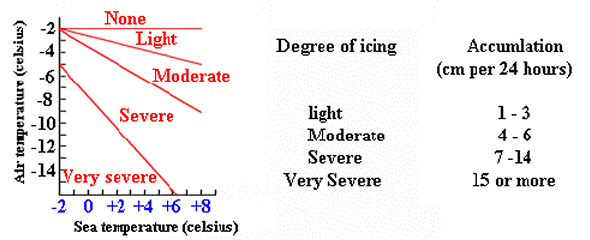
Figure 5.2: A Mertins diagram over icing vs. sea and air temperature with wind of gale force. Similar diagrams must be used for other ranges of wind speeds

Impressions of the polar low on the ground

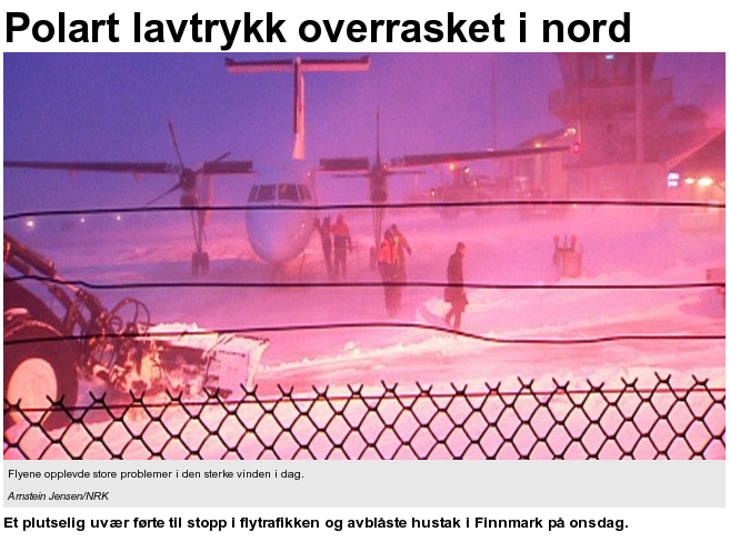
Figure 5.3: Cancelled flight due to a polar low in Hammerfest. Business no longer as usual... Photo: Arnstein Jensen/NRK

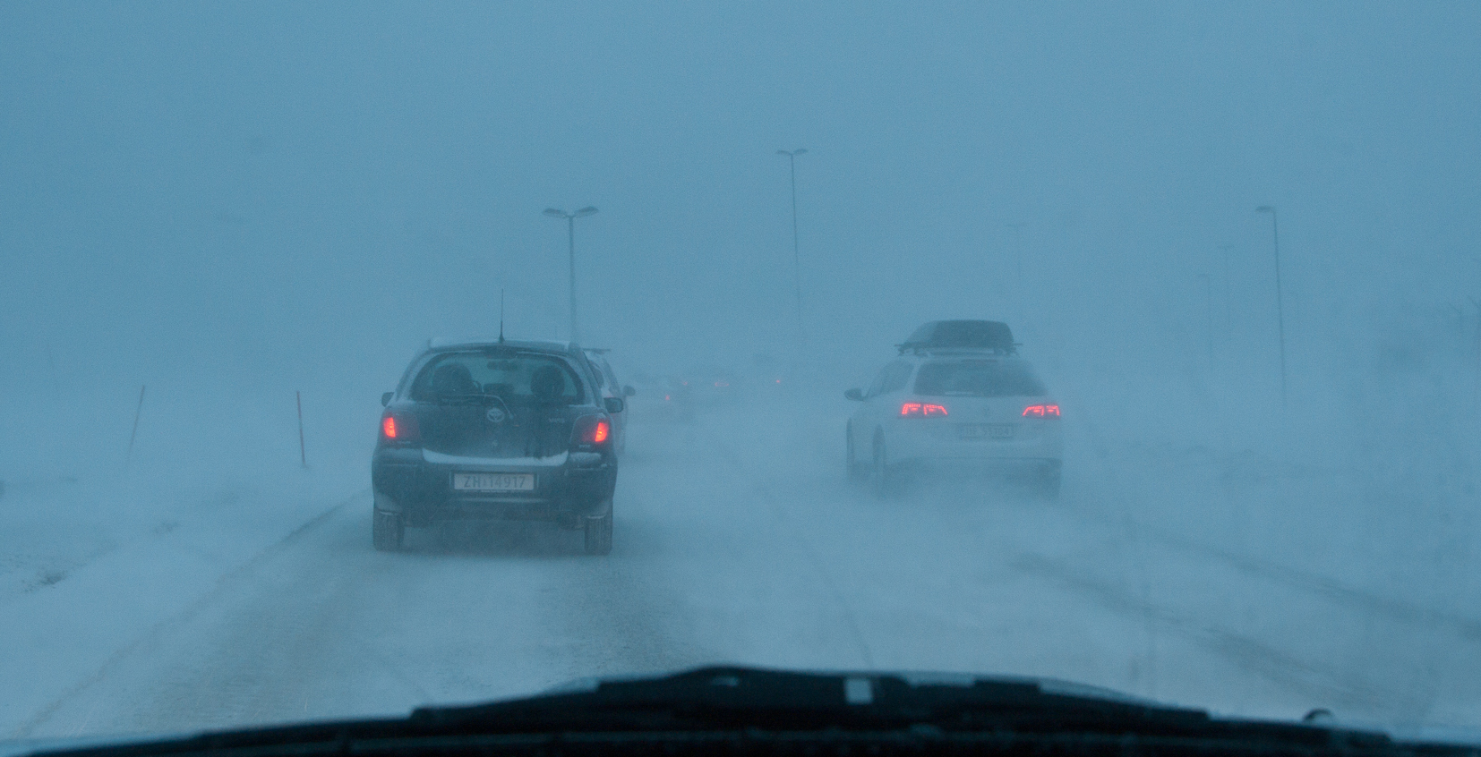
Figure 5.4: A combination of wind, windblown snow and and heavy snowfall gives severely reduced visibility and often very difficult driving conditions as Polar Lows make landfall. Disruption of both marine and air traffic is common. Photo: Gunnar Noer

Figure 5.5: A polar low as seen from the inside, the eyewall approaching. Photo: Gunnar Noer

This shear zone is the reason why polar lows are feared in the coastal fisheries. The wind is commonly reported to increase from calm to storm force winds in less that 10 minutes. Waves are observed to increase rapidly in a similar time span, with difficult and confused wave conditions as a result of rapidly changing wave and wind directions.

 

References

Blechschmidt, A.-M., 2008: A 2-year climatology of polar low events over the Nordic seas from satellite remote sensing. Geophys. Res. Lett., 35, L09815, doi:10.1029/2008GL033706.

Businger, S. (1985), The synoptic climatology of polar low outbreaks, Tellus, Ser. A, 37, 419-432.

S. Bakan, and H. Graßl, 2009: Large-scale atmospheric circulation patterns during polar low events over the Nordic seas. J. Geophys. Res., 114, D06115, doi:10.1029/2008JD010865.

Bracegirdle, T. J., and S. L. Gray, 2008: An objective climatology of the dynamical forcing of polar lows in the Nordic seas. Int. J. Climatol., 28, 1903-1919, doi:10.1002/joc.1686.

Condron, A., G. R. Bigg, and I. A. Renfrew, 2006: Polar mesoscale cyclones in the northeast Atlantic: Comparing climatologies from ERA-40 and satellite imagery. Mon. Wea. Rev., 134, 1518-1533, doi:10.1175/MWR3136.1.

Erik W. Kolstad (2006) A new climatology of favourable conditions for reverse-shear polar lows, Tellus A: Dynamic Meteorology and Oceanography, 58:3, 344-354, DOI: 10.1111/j.1600-0870.2006.00171.x

Laffineur, T., C. Claud, J.-P. Chaboureau, and G. Noer, 2014: Polar lows over the Nordic Seas: Improved representation in ERAInterim compared to ERA-40 and the impact on downscaled simulations. Mon. Wea. Rev., 142, 2271-2289, doi:10.1175/ MWR-D-13-00171.1.

Mallet, P.-E., C. Claud, C. Cassou, G. Noer and K. Kodera (2013), Polar lows over the Nordic and Labrador Seas: Synoptic circulation patterns and associations with North Atlantic‐Europe wintertime weather regimes, J. Geophys. Res. Atmos., 118, 2455-2472, doi:10.1002/jgrd.50246.

Noer, G., and T. Lien, 2010: Dates and positions of Polar Lows over the Nordic Seas between 2000 and 2010. Norwegian Meteorological Institute Rep. 16/2010, 7 pp.

Orimolade, A. P., B. R. Furevik, G. Noer, O. T. Gudmestad, and R. M. Samelson(2016), Waves in polar lows, J. Geophys. Res. Oceans, 121, doi:10.1002/2016JC012086.

Rojo, M., Claud, C., Mallet, P.E., Noer, G., Carleton, A.M., Vicomte, M. (2015): Polar low tracks over the Nordic Seas: a 14-winter climatic analysis, Tellus A: Dynamic Meteorology and Oceanography, 67:1, DOI: 10.3402/tellusa.v67.24660

Rasmussen, E., and J. Turner, 2003: Polar Lows: Mesoscale Weather Systems in the Polar Regions. Cambridge University Press, 612 pp.

Saetra, Ø., Noer, G., Lien, T., Gusdal, Y., 2011: A climatological study of polar lows in the Nordic Seas. Quart. J. Roy. Meteor. Soc., 137, 1762-1772, doi:10.1002/qj.846.

Smirnova, J. E., P. A. Golubkin, L. P. Bobylev, E. V. Zabolotskikh, and B. Chapron, 2015: Polar low climatology over the Nordic and Barents Seas based on satellite passive microwave data. Geophys. Res. Lett., 42, 5603-5609, doi:10.1002/2015GL063865.

Saetra, Ø. Noer, G., Lien, T. Gusdal, Y., STARS-DAT (2013), STARS Data Set, Oslo, Norway. [Available: http://polarlow.met.no/stars-dat/, accessed 13 December 2015.]

Terpstra, A., C. Michel, and T. Spengler, 2016: Forward and reverse shear environments during polar low genesis over the northeast Atlantic. Mon. Wea. Rev., 144, 1341-1354, doi:10.1175/MWR-D-15-0314.1.

Tilinina, N., S. K. Gulev, and D. H. Bromwich, 2014: New view of Arctic cyclone activity from the Arctic system reanalysis. Geophys. Res. Lett., 41, 1766-1772, doi:10.1002/2013GL058924.

Wilhelmsen, K., 1985: Climatological study of gale-producing polar lows near Norway. Tellus, 37A, 451-459, doi:10.1111/j.1600-0870.1985.tb00443.x.

Zahn, M., and H. von Storch, 2008: A long-term climatology of North Atlantic polar lows. Geophys. Res. Lett., 35, L22702, doi:10.1029/2008GL035769.

Zappa, G., L. Shaffrey, and K. Hodges, 2014: Can polar lows be objectively identified and tracked in the ECMWF operational analysis and the ERA-Interim reanalysis? Mon. Wea. Rev. ,142, 2596-2608, doi:10.1175/MWR-D-14-00064.1.