Meteorological Physical Background
Size of the Polar Low
Polar Lows develop within small baroclinic disturbances in a potentially unstable environment north of the polar front in the marine Arctic. The small scale of the Polar Low can be explained with the Rossby radius of deformation: R~N0H/f. In this equation, f is the coriolis parameter, N0 is the stability parameter, H is the scale height and R is the minimum scale of a system to be dynamically stable. The saturated-adiabatic lapse rate (small N0), the northern position (large f) and very cold air mass (small H), result in an R being significantly smaller in a Polar Low environment than in an environment of an extratropical cyclone.
Developing phase, necessary conditions
A polar low usually forms as a consequence of both baroclinic and static instability, the latter being almost unobstructed from low levels and up to above 500 hPa. In addition, also PVA at upper levels needs to be present. In the developing phase, the following elements are most common:
- There needs to be a marine cold air outbreak (MCAO) at low levels within a marine mixed layer (MML). This layer is destabilized by supply of felt and latent heat from the ocean surface. The MML extends upwards to the inversion initially created by the cooling of the lower air mass as it passes over ice and snow covered surface. The top of this inversion is typically at 3 to 5 km height.
- There needs to be a cold air mass above the MML, and an unstable stratification from the inversion layer at the top of the MML and up to at least 500 hPa. The rapid intensification of a Polar Low takes place when the MML is heated sufficiently so that the inversion layer above the MML is broken down and unobstructed static instability all the way up to above 500 hPa is achieved.
- Positive vorticity advection (PVA) is supplied by an upper trough, most easily seen from the geopotential in 500 or 300 hPa. In the context of a polar low, there are usually quite low values of PVA, associated with a slow moving upper trough, but acting over a longer time period.
- There needs to be an area of enhanced baroclinicity at low to middle levels that can, under influence of the upper trough and together with static instability, intensify into a Polar Low. The baroclinic zone can have different origins. Most commonly it is: 1) a remnant of an old occlusion, 2) a convergence zone, e.g. the one that often forms south of the tip of Spitsbergen in a northerly flow, or 3) at the fringes of a cold air outbreak, between the cold air in the north and warmer air to the south.
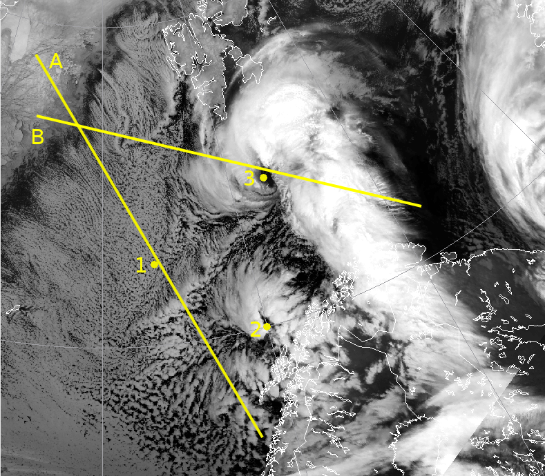
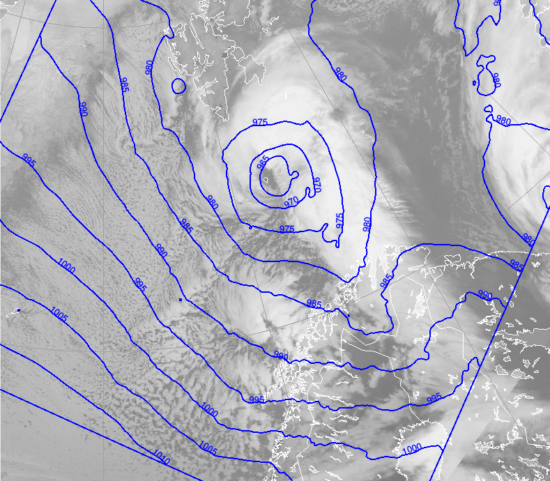
Figures 2.1a-d shows an example of a Polar Low and a cold air outbreak from 19th of January 2017 at 09Z, as seen with 0Z run from the Arome-Arctic 2,5km NWP model used at MET-Norway: In the upper left figure is the plain IR image, with cross sections and sounding points indicated. The main center is lying directly over Bear Island, and is moving in an easterly direction. The CAO is from the Fram strait west of Spitsbergen and the East Greenland ice cap. As the air leaves the ice, there is initially homogeneous convection with tops gradually increasing downstream. Approaching the Norwegian coast there is a cluster of enhanced convection and a small Polar Low. The upper right image shows the corresponding impression in the MSLP; a well defined closed low center, in this case almost symmetrical. The pressure pattern implies a strong northwesterly winds from the Greenland ice and an ongoing CAO.
 |
 |
 |
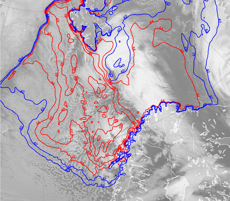 |
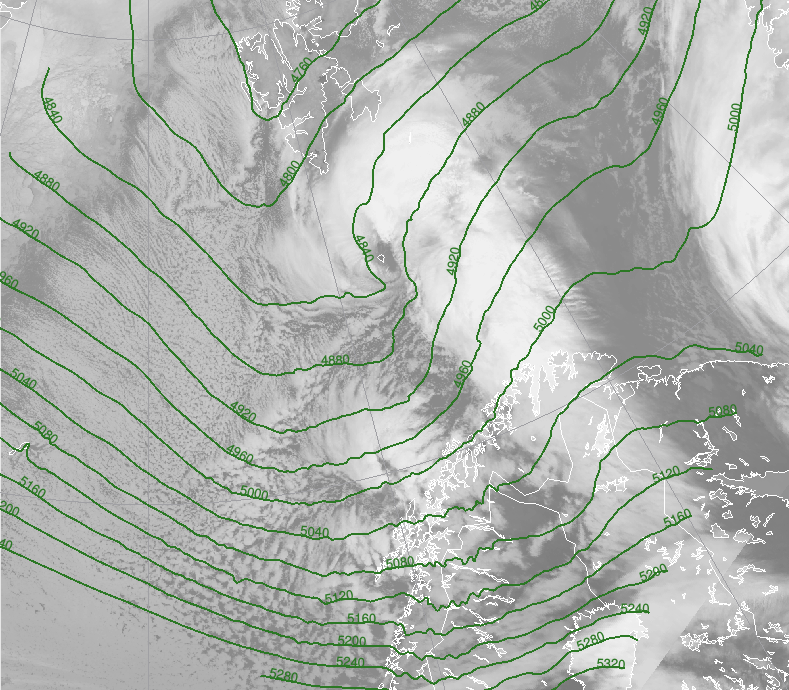
Figure 2.1: Four panes showing an example of parameters from the Polar Low from 19 January 2017 at 09 UTC. Illustration: MET/NOAA
The bottom left image shows a typical upper trough as seen in the Z500 geopotential, with a rather wide extent. Bottom right shows the SST-T500, which corresponds well in extent with the convective area. The main low is here situated in an area of steep gradient in the SST-T500, indicating that some baroclinic instability is present. The southern minor low is associated with an area of high values of SST-T500, so this low is mainly driven by deep static instability.
 |
 |
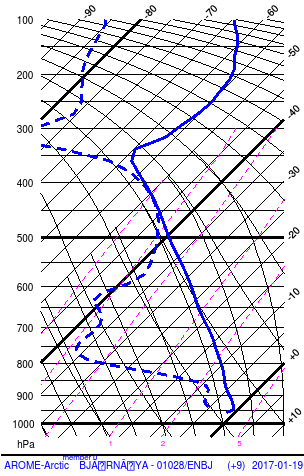 |
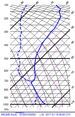
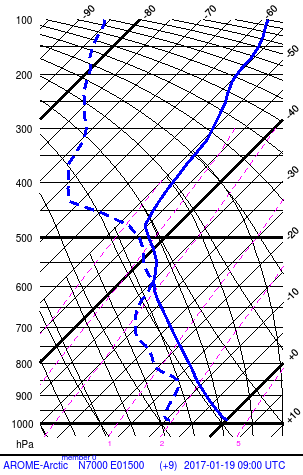
Figure 2.2: Figure 2.2: Soundings from point 1, 2 and 3 (left to right) in figure 2.1. Illustrations: Noer/MET
Figure 2.3 shows a cross section along line A. The marine mixed layer (MML) increases gradually in depth from the ice edge to the Norwegian coast where it attains a maximum height of 4000m (600 hPa), but the inversion on top of the MML is still not broken down. The left sounding in figure 2.2 is from point 1, midway along line A, and is typical for shallow convection with a strong inversion at the top, in this case at 3 km (700 hPa) height.
The sounding in point 2 is taken slightly northeast of line A, at an area with more deep convection. The main inversion here is at 6 km (500 hPa), consistent with the small polar low forming here. A lesser inversion at 600 hPa is at the same level as the top height of the MML seen at the southeastern end of line A. As can be seen from the cloud mass of the satellite image in figure 2.1a, this slight inversion is sufficient to stop the convection from reaching higher.
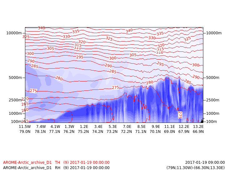
Figure 2.3: Cross section A across a CAO with moderate vertical extent. Red lines are potential temperature. Blue shading are relative humidity. Illustration: Noer/MET
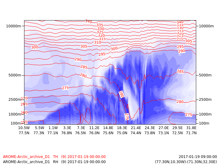
Figure 2.4: Cross section B across a polar low. Red lines are potential temperature. Blue shading are relative humidity. Illustration: Noer/MET
Figure 2.4 shows the cross section B through the polar low. The inversion is broken down around the center (east of 14E), and the moisture and clouds are transported up by convection to the tropopause at 7 km (400 hPa) height. The sounding at point 3 is at the center of the main Polar Low. The air column is unstable up to the tropopause at 400 hPa, and typically polar lows form in air masses where the tropopause is between 500 and 400 hPa. Comparing to the sounding at point 2, we see that the air mass above 500 hPa is colder at point 3, - there is an upper cold core present.
Synoptic situation, reversed or direct shear
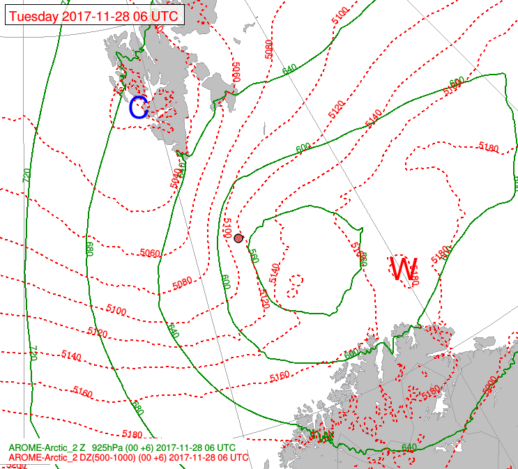
Polar Lows often form in a northerly flow behind a major synoptic low, with the low center to the south or east but the cold air to the north or west of the center. In such cases the thermal wind is in the opposite direction of the pressure gradient wind, and the wind will decrease and shift direction with height. This condition is called reversed shear, and is most common with polar lows. In this condition the upper trough is positioned above or ahead of the surface low, as opposed to the 'normal' direct shear case where the upper trough is trailing the surface low. Another feature often seen in reversed shear cases is that the reduction in wind speed in the vertical tends to be concentrated in a shear zone around the 850 to 700 hPa level. The steering level of the polar low is then found at the top of the bottom level, just below the shear zone.
 |
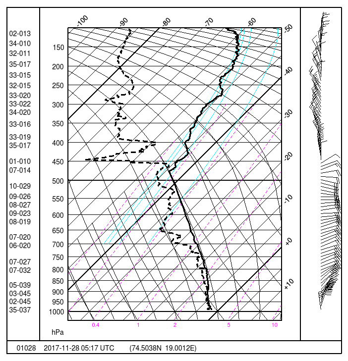 |
Figure 2.5: Reversed shear seen in a polar low from 17th November 2017.
Left image shows the geopotential in 925 hPa (green) and 1000 - 500 hPa thickness (red). In this case, the strongest gradients is in the area near Bear Island (red dot). The gradient in the thickness is in the opposite direction of the pressure gradient, hence the thermal wind acts to decrease wind with height. The right image shows the corresponding sounding from Bear Island. Wind direction and speed (knots) is given by the numbers on the far left in the sounding. In this case, the strongest wind is found at 900 to 950 hPa.
Spatial distribution of Polar lows
The amount of static instability in the MML is closely coupled to the supply of latent and felt heat from the sea surface, which in turn is dependent on the difference in the temperature of the air close to the sea surface and the sea surface itself. This is largest close to the ice edge, where the difference can be of more than 40°C, but of more importance is the difference further downstream as the cold air is advected over the warmer waters of the North Atlantic current. Especially where the air mass is advected across areas of steep gradients in the sea surface temperature (SST), e.g. at the edges of the various branches of the North Atlantic current, the airmass is prone to develop deep convection and polar lows. As can be seen from illustration 2.6, the polar lows mainly develop over the warmer areas of the North Atlantic.
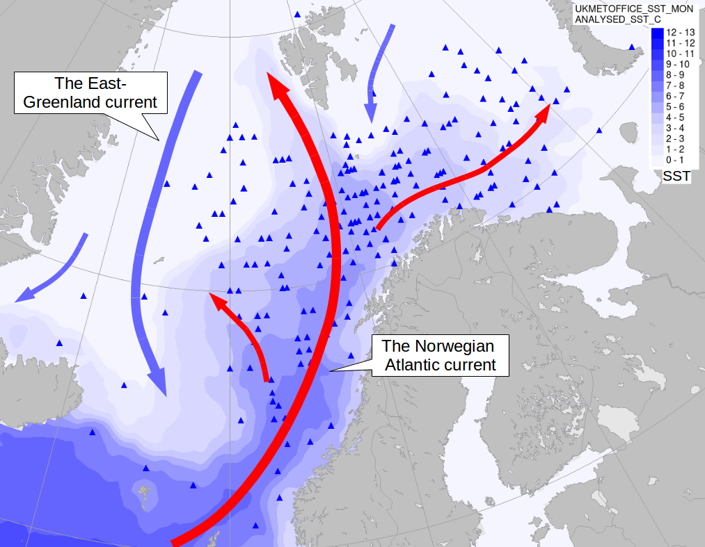
Figure 2.6: The genesis areas of polar lows from 2000 till 2017 plotted as triangles. Blue shading is monthly mean sea surface temperature in February (UK MetOffice). Also shown are the main ocean currents in the North Atlantic, showing the sourced of warm and cold water in the area. Illustration: Noer/MET
There is a slightly higher concentration in the area south of Bear Island. This is probably because this area receives CAO from both sides of Spitsbergen, as well as being subjected to convergence and enhanced convection off the south tip of Spitsbergen in northerly flow. There are less Polar Lows in the eastern part of the Barents sea because the SST and also gradients in SST are less in this area.
Because of the significance of the SST, to identify the cold cores that favor growth of polar lows it is more useful to consider the difference between SST and the temperature at 500 hPa. In earlier years when the location of the cold cores was uncertain, it was common to consider the max value of this difference, and a threshold of 44°C was used to indicate an area prone to PL development. In recent years, and especially when using the SST - T500 difference e.g. for automated tracking, the difference is taken in the same gridpoint. In such cases a lower value must be used, and 40°C is now considered to be the most appropriate.
This is also physically consistent with the fact that most polar lows develop as a result of a mix of static and baroclinic instability, and a common source of the latter is at the edges of the cold air outbreaks, between the cold and warm air masses, but where the temperature at 500 hPa is not as low as at the center of the cold core.