Cloud Structure In Satellite Images
Appearance In Satellite Data
Polar Lows are small, but fairly intense maritime cyclones that form poleward of the polar front (Rasmussen and Turner, 2003). The horizontal scale of the polar low is approximately 150 to 600 kilometers, and sustained wind at 10 meter height is near or above gale force (>13,8 m/s). On average, maximum observed wind is at 22 m/s. Polar lows are a wintertime phenomenon that occurs mainly from October until April. Because of their northerly position, their small scale and their appearance in the dark winter season, AVHRR IR or day/night channel 3-4-5 images are the best way to detect Polar Lows. At latitudes lower than 68 degrees north, Meteosat IR are also useful for detecting such systems.
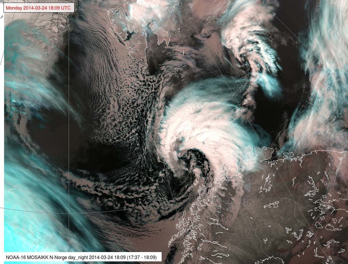
Figure 1.1: A mature Polar Low off the coast of Finnmark in Northern Norway from late March in 2014. This image is a combination of channels 3, 4 and 5, commonly known as the 'day/night combination. White is high and cold clouds. Grey is low/warm clouds. Black is sea. Blue/greenish is cirrus or high ice clouds. Illustration: MET-Norway/NOAA
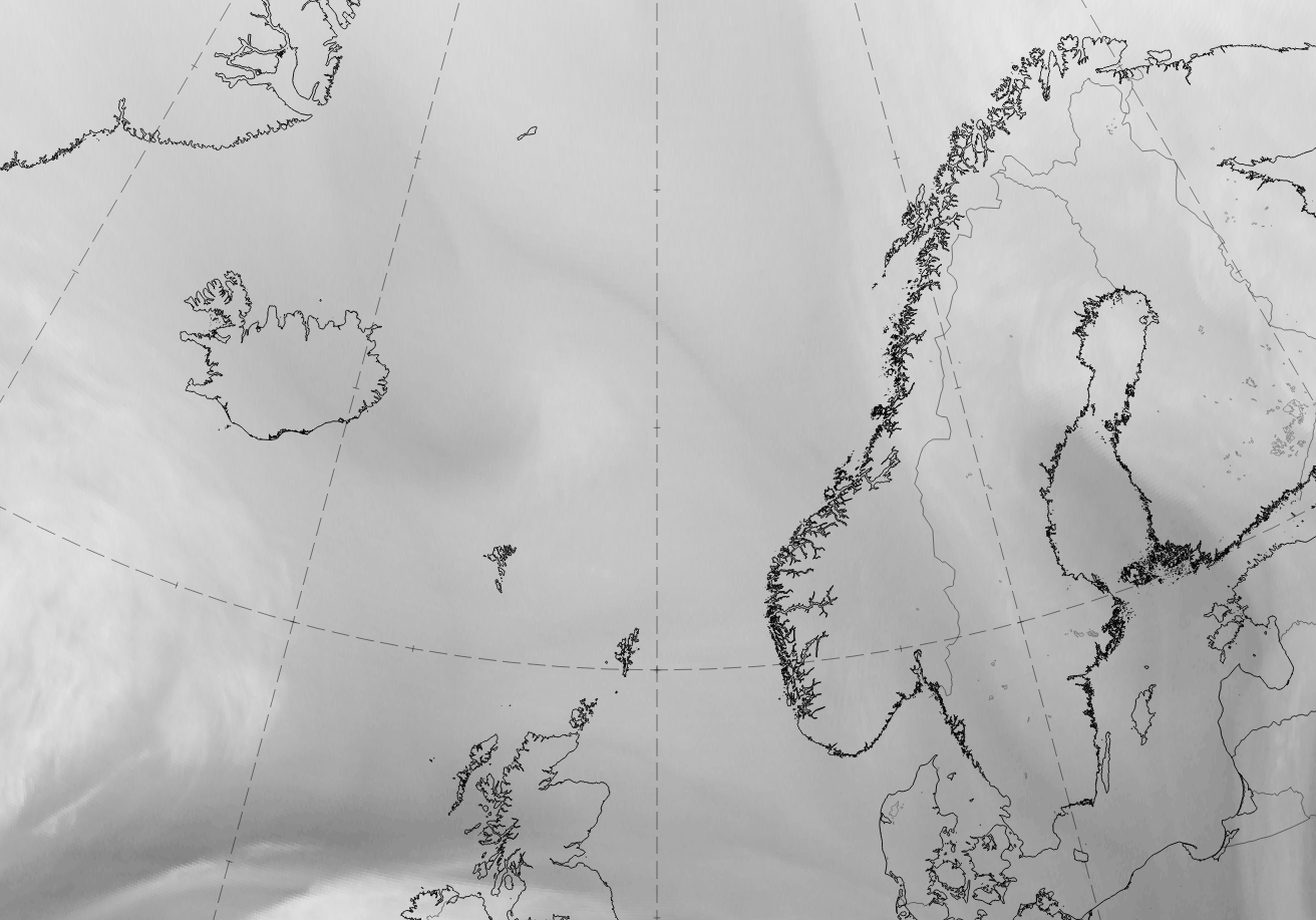
As can be seen from the various pictures in this section, the typical shape of the Polar Low is that of a non-symmetrical small cyclone around a dark and nearly cloud free eye. Normally there is an opening in the cloud mass south of the center. In the northern to eastern part there is a high and smooth cirrus shield, but in some cases with bands of convection is seen in this area. To the left of center is the tip of the cloud band, often with lower cloud top temperatures indicating that there is some descending motion here. This area is where the strongest winds are located around the low. Frequently also a wavelike feature can be seen at the western or northern edge of the cloud mass, indicating shear between the circulation around the low and an overlying jet.
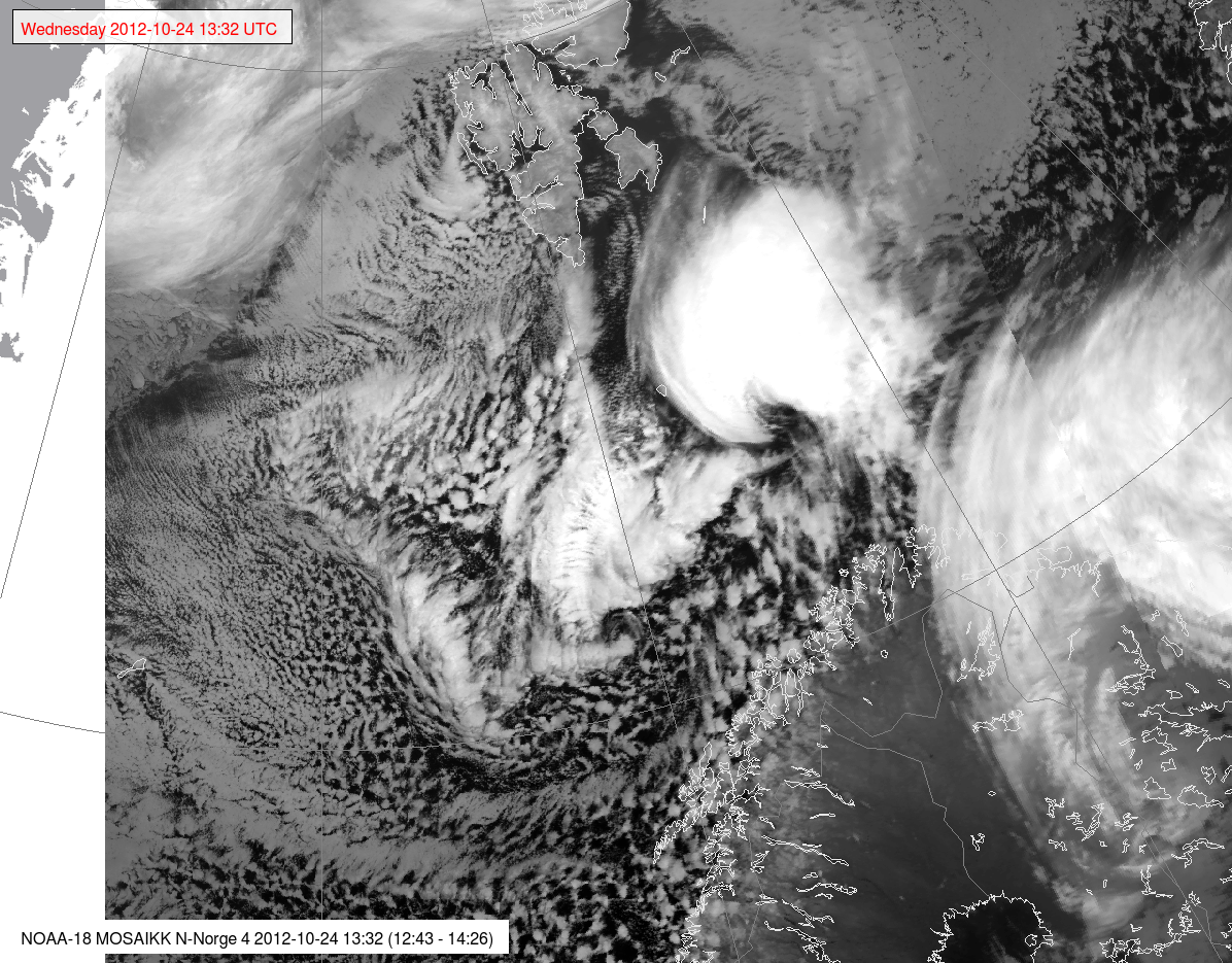
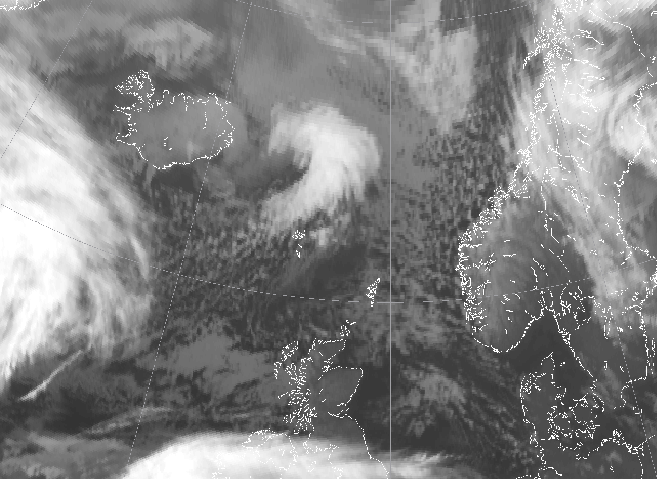
Figure 1.2: IR-image of a mature polar low southeast of Bear Island. To the southwest of this is a smaller low in its developing phase, and still further southwest is a north-south oriented trough where some cyclonic curvature and an emerging eye can be seen. Illustration: MET-Norway/NOAA
Polar lows is most common in the Norwegian Sea and the Barents sea, mainly east of the 0-meridian, and between 65 and 76 degrees north, but cases are known all the way south to the North Sea coast of continental Europe. Another area with high occurrence is to the south and east of the south tip of Greenland. These lows can usually be classified as lee lows or comma clouds in an easterly moving air mass, and do mainly affect the waters around the British Isles and the North Sea. The Japan Sea is known to be a prolific area for polar low formation. The Hudson Bay has some cases in the ice free autumn season, manly in October and November. There are also Polar Lows in the Antarctic, but since winds here are mainly zonal, cold air outbreaks from the ice is less persistent, and PL's here are generally weaker than those found in the Arctic.
Three different phases in the life cycle of a Polar Low can be distinguished: the initial/development phase, the mature phase and the decaying phase. It is also useful to consider the cold air outbreak since this is a necessary precursor for Polar Low formation.
The cold air outbreak
Polar lows are uniquely associated by cold air outbreaks (CAO) from the polar ice, and the CAO can be seen as a precursor to PL formation. Cold air outbreaks can easily be seen from satellite imagery. As the cold air flows out over open water, convection forms along lines oriented in the direction of the air flow in so called 'cloud streets'. These form a very intuitive impression of the flow in the mixed layer.
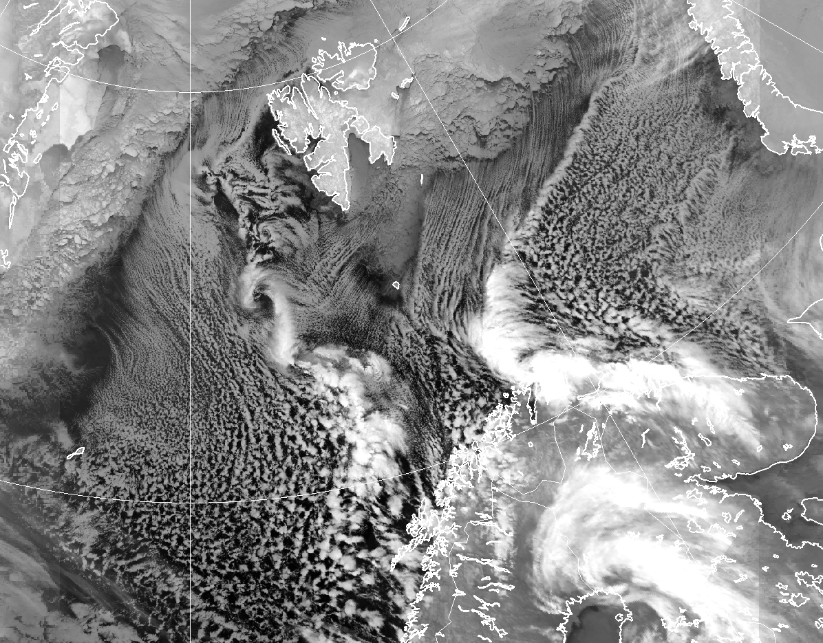
Figure 1.3: A cold air outbreak from March 2013. Cloud streets are clearly visible, as well as two convergence lines. The flow is generally in a southerly direction, and both convergence lines develop into very deep convection as they approach the Norwegian coast. illustration: MET-Norway/NOAA
Convergence lines forms where air masses meet, and these are prone to intensify into polar lows or other deep convection. In figure 1.3 a mature CAO is shown extending from Greenland till Novaya Zemlya. The wedge shape of Spitsbergen is particularly effective in modifying the flow to converge in the areas around Bear Island.
The developing phase
A developing Polar Low has the structure of a cyclonic curl that emerges from an otherwise more unorganized cloud mass, e.g. an old occlusion, a Cb-cluster or a convergence zone. Surrounding the emerging cyclone are cloud streets of shallow convective clouds with relatively low tops (darker grey in IR), typical for a cold air outbreak. The inner part of the curl shows sharp cloud edges while the outer part is often capped by cirrus cloud with fussy edges.
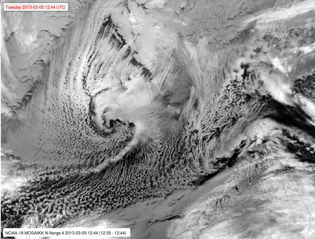
Figure 1.4: An Arctic front or convergence line extending westwards from Spitsbergen is curling up and starting to grow into a Polar Low. The eye and the cyclonic curvature is what distinguishes it from a trough or convergence line. Very white clouds west of Spitsbergen shows that this air mass is very cold and has potential for deep convection and Polar Lows. Illustration: MET-Norway/NOAA.
Mature stage
The cloud structure of a mature Polar Low is often a pronounced vortex with a (partly) cloud free and warm eye. The eye consists of relatively warm subsiding air at the center of the low, and it shows up dark or almost black in the IR image. Surrounding the eye is a continuous area of deep convection with strong vertical updraft and with heavy precipitation. This extend all the way up to the tropopause, which can be quite low in polar low situations, typically at 5 to 7 kilometers. Under the tropopause, the ascending air spreads out in a smooth cirrus shield that appears as bright white in the IR images. In some cases can be seen wavelike ripples extending out at the fringes of the cirrus shield. These indicate that there is an overlying jet and a wind shear at the top of the convective layer. Clouds at the 'tip' of the spiral tend to be less bright, indication tops at a lower level and that there are descending motion in this area.
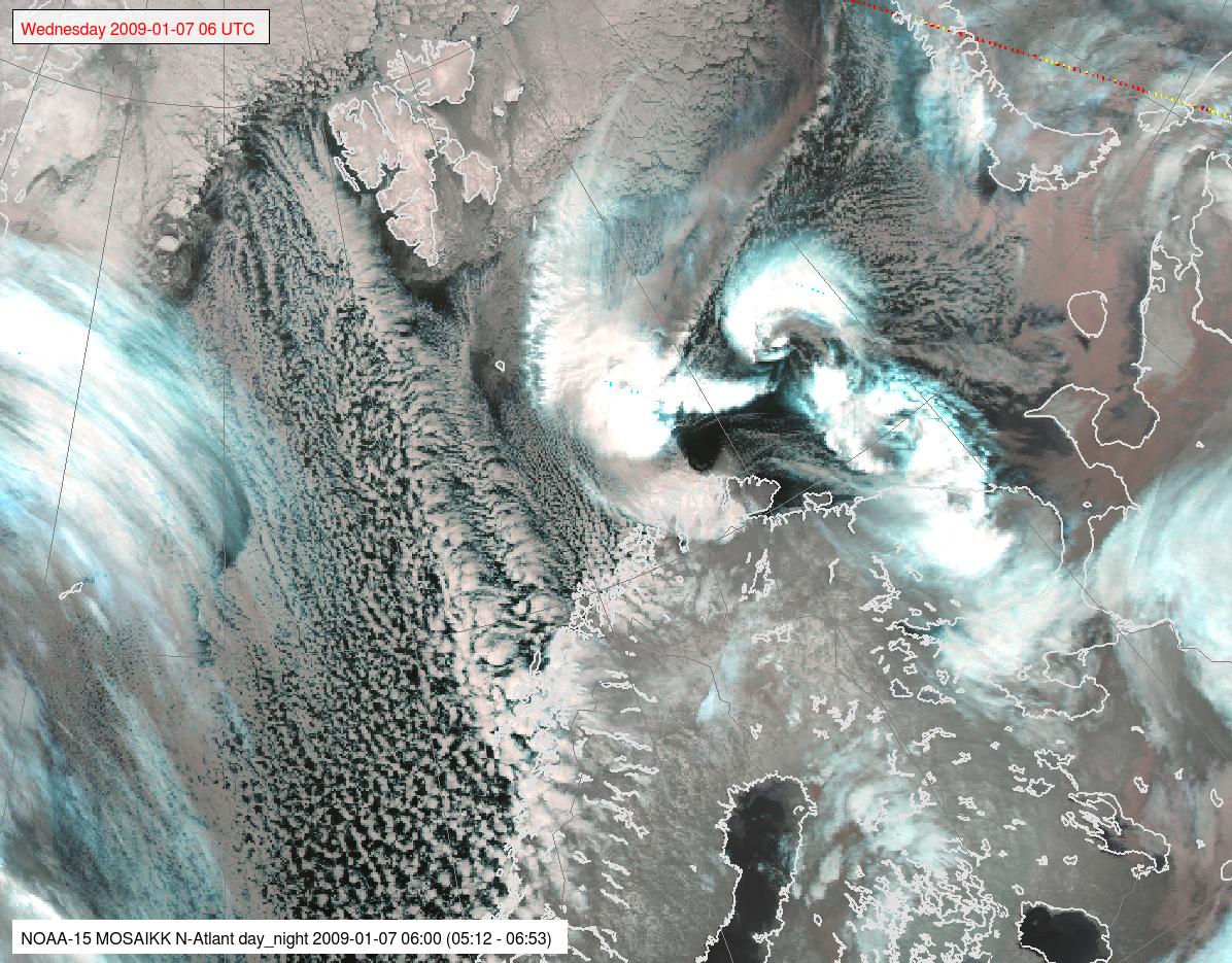
Figure 1.5: A mature polar low hitting the coast of Finnmark in January 2009. The eye can clearly be seen, as well as the smooth cirrus shield on top. Quite often polar lows appear in clusters of two or more, in this case there are two smaller eddies east of the main center. Illustration: MET-Norway/NOAA
Decaying phase
The most common reason for dissipation is that the low makes landfall. When the energy source from the warm sea is cut off and the low moves in over cold and dry land, it quickly loses its momentum.
 |
 |
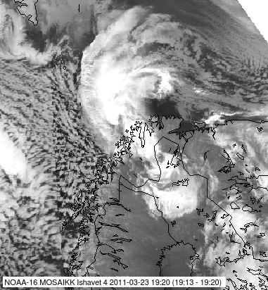 |
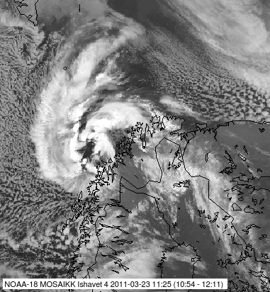
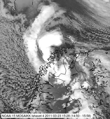
Figure 1.6: A Polar Low from march 2011 at different stages of landfall dissipation. To the left is at mature stage over open waters. Middle is just after landfall. The wind has subsided, but heavy precipitation is still present. On the right only high clouds remains. Although the cyclone can still be seen, the low has little impact on surface weather at this stage. Illustration: MET-Norway/NOAA
Negative vorticity advection is another effective way to weaken a low; the upper trough moves off and is replace by a ridge. In such cases the convection dissolves into more stratiform cloud types. An approaching warm front will also act to stabilize the air column, and will effectively stop a Polar Low in its development. From AVHRR images the low simply seem to vanish under the leading edge of the frontal clouds, and it soon loses its strength also at the surface.
Frequently a polar low dissipates while still over open water. Often the best sign of this kind of dissipation is that the cloud pattern becomes more disorganised. The cirrus is less visible or absent, and more is seen of the Cb cells or bands of convection at lower levels. These have a more chaotic flow under the cloud base, as opposed to the well organized inflow that exists at low levels around a mature polar low.
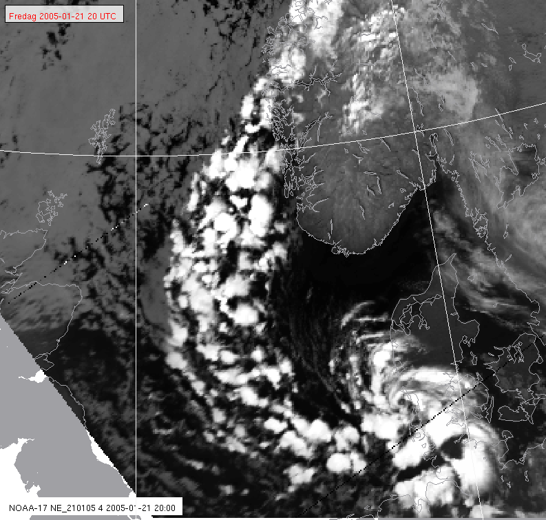 |
Figure 1.7: A decaying polar low hitting the coast of Denmark in January 2005. The cirrus shield is gone, and individual Cb cells can clearly be seen. There is still some cyclonic curvature in the band of Cb's. This low will still give gale force winds and quite heavy precipitation. Illustration: MET-Norway/NOAA |
Meso circulations and shallow polar lows
There are low pressure systems that have similarities to a polar low, but that are less intense and have less impact on the surface weather. Inspection of satellite imagery can give important information on the nature of these lows and help assess the depth of these lows.
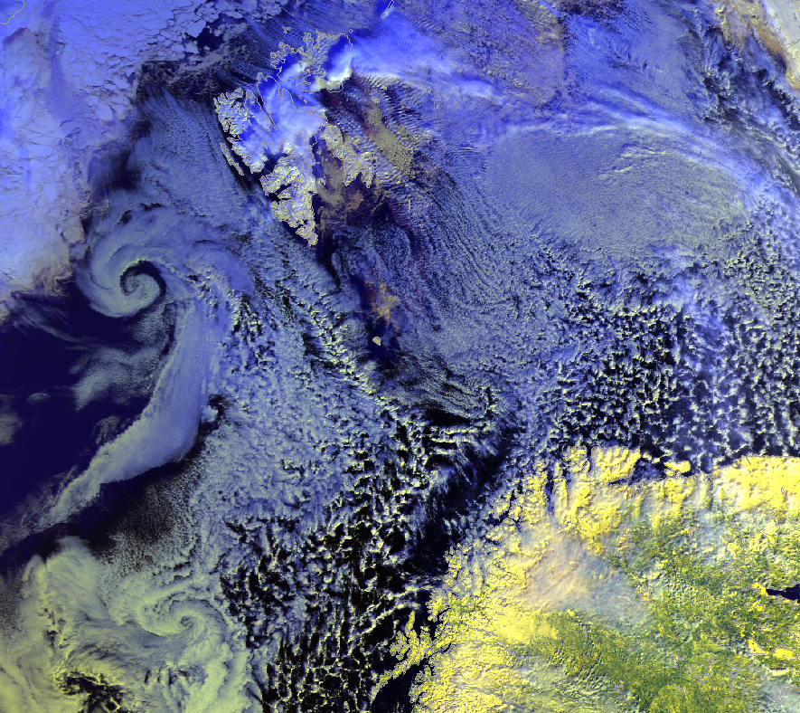
Figure 1.8: A meso circulation southwest of Spitsbergen on the 31st March 2014. Illustration: MET/NOAA
Illustration 1.8 shows a typical meso circulation southwest of Spitsbergen. The low brightness of the cloud and the fact that this is the same as that of the clouds surrounding it indicates that this low is not penetrating through the inversion above the Marine Mixed Layer (MML). Also, it has a smooth appearance of stratiform clouds at the top, but no cirrus. Hence this is a shallow low, often called a 'Meso Circulation', where the convection is confined to the mixed layer. Such lows usually have limited impact of one to two Beaufort on the surface wind.
In some cases very strong wavelike cloud patterns can be seen around the periphery of the cloud mass of the low, as shown in the example below. This indicates that there is a strong capping inversion and strong windshear above this, typically from an overlying jet. In the example shown, the flow in the MML was northeasterly, but above this there was a northwesterly jet. The ripples are waves in the shear zone between the to layers. Although it looks dramatic, this is usually a sign of a moderate vertical extent and moderate impact on the surface weather.
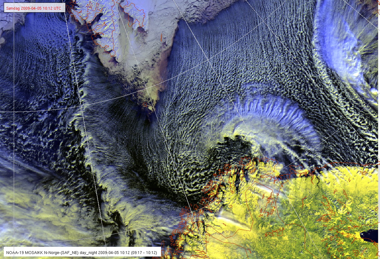
Figure 1.9: A shallow polar low north of the Finnmark coast, with unusually large wavelike cloud pattern around the center. Illustration: MET-Norway/NOAA
Appearance in geostationary Meteosat imagery
 |
 |
 |
 |
 |
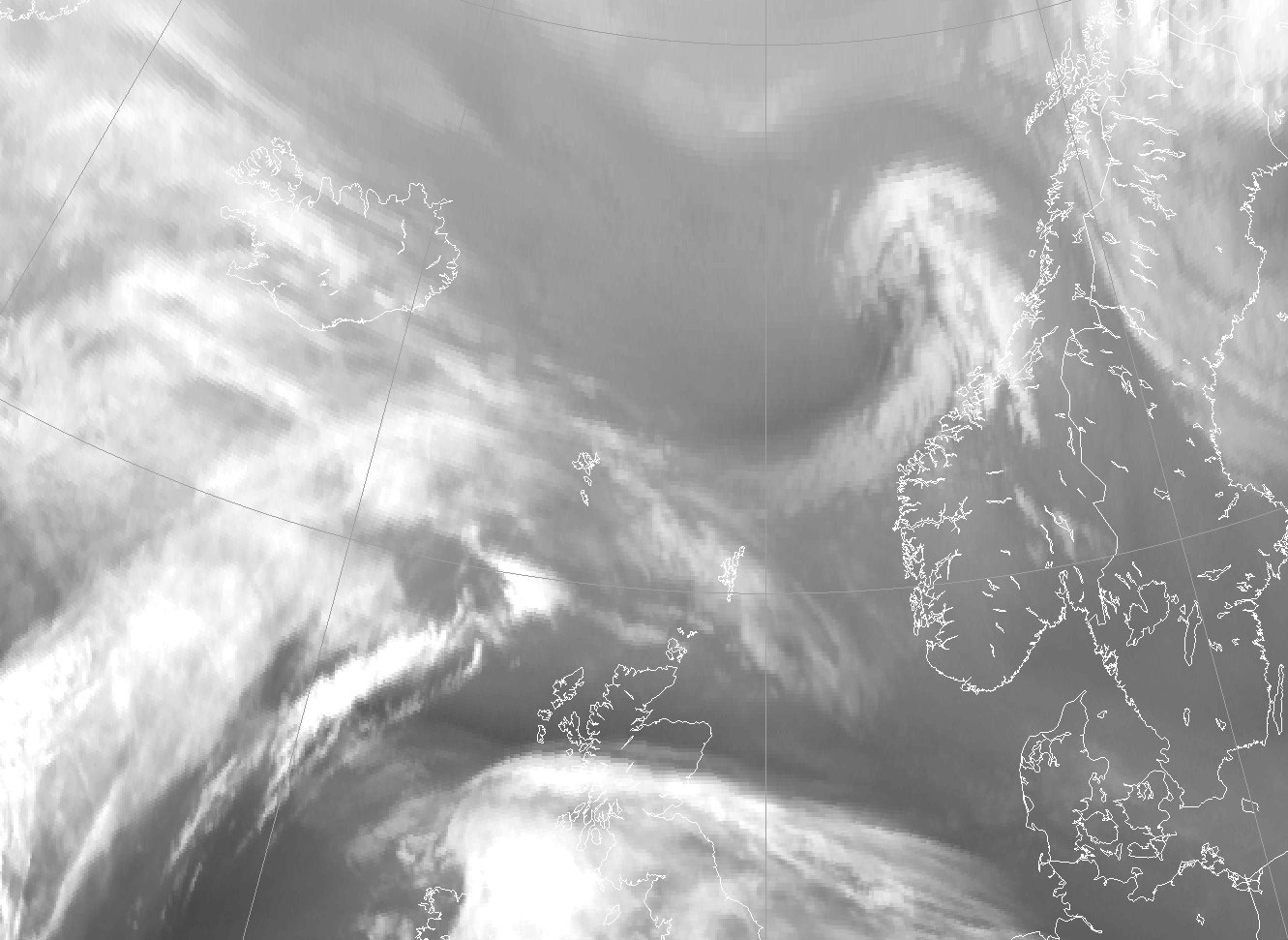 |
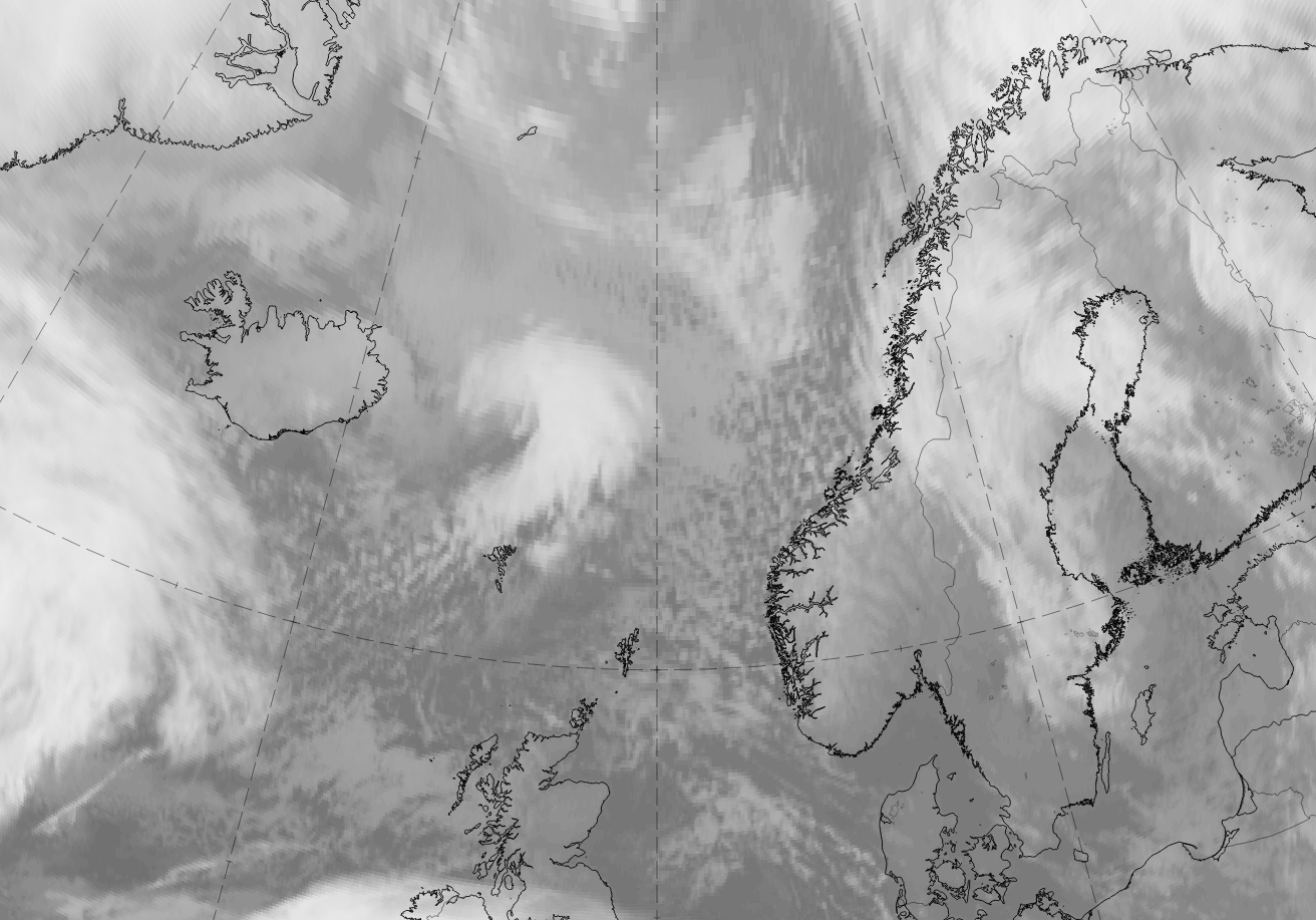
Figure 1.10: Meteosat images of a forming polar low east of Iceland on 4 December 2018
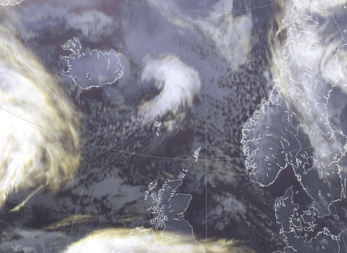
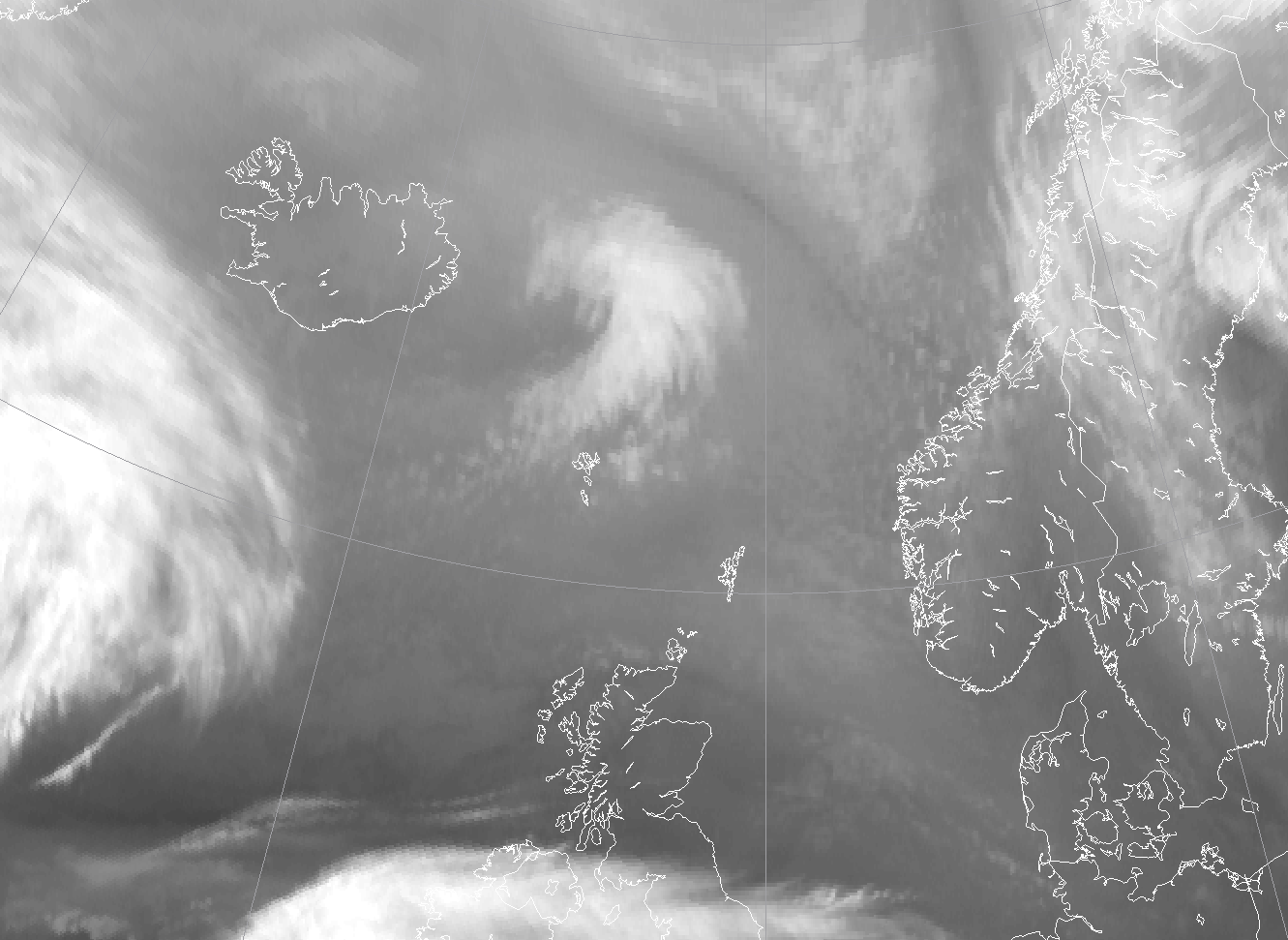
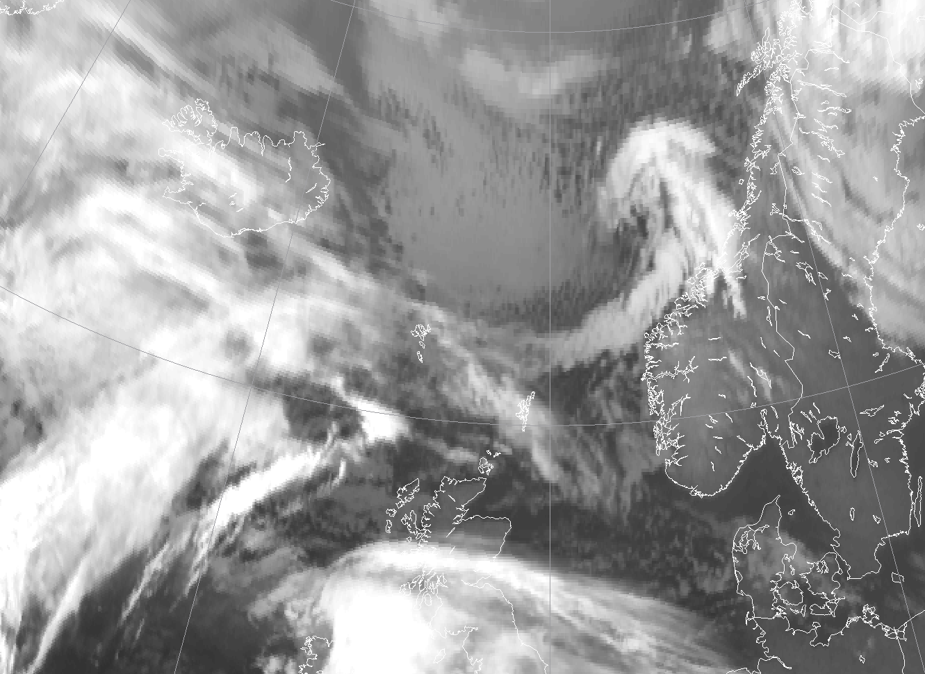
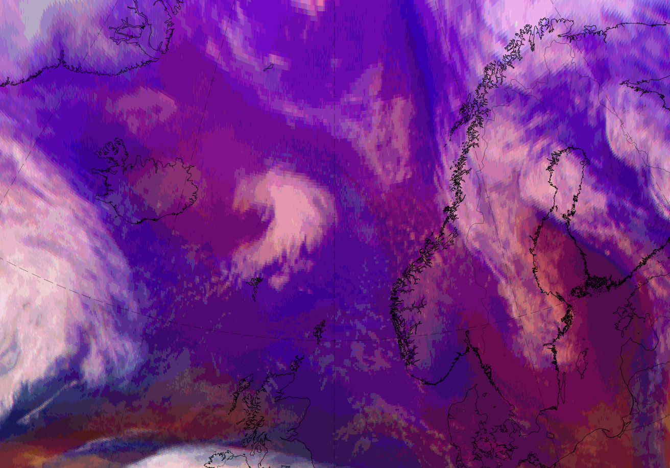
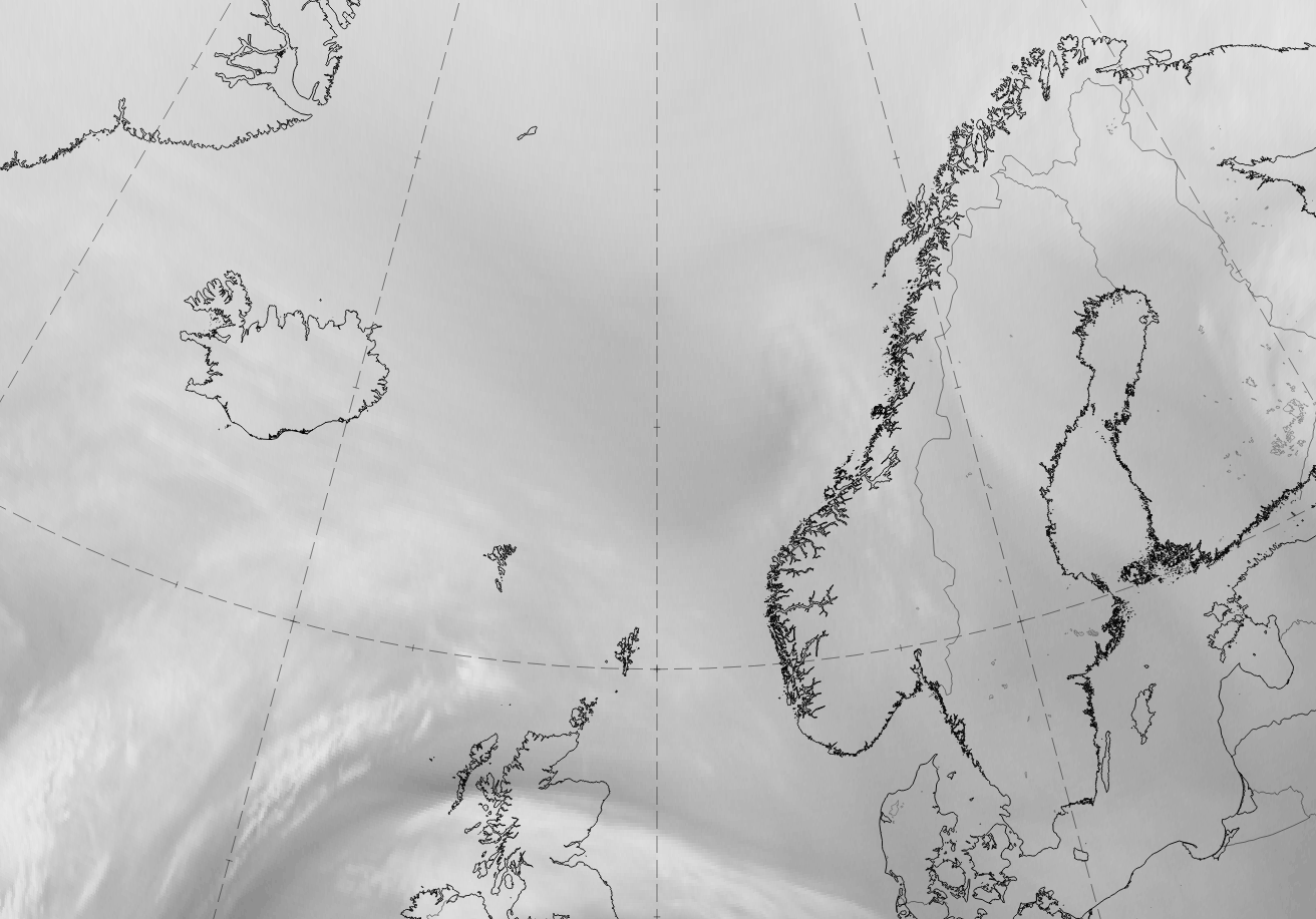
If the Polar Low is not too far to the north, it is possible to trace it with Meteosat images. In the first row above, a Comma shaped Polar Low is developing east of Iceland on the 4 December 2018. The left IR image shows the mature stage in IR channel 10,8, then the combination IR12.0, IR10.8 and IR3.9, and to the right the water vapour channel WV7.3. In the lower row can be seen the low at a later stage, just before landfall at the coast of Norway. From the dark areas in the WV channel can be seen that there are some tropopause folding associated with this low, indicating a frontal structure in the cloud bands around the center. Comma clouds in southwesterly flow is common in the central North Sea, often having an origin as a lee wave off the south tip of Greenland. These often have a stronger similarity to baroclinic synoptic low than the more convectively driven polar lows further north.
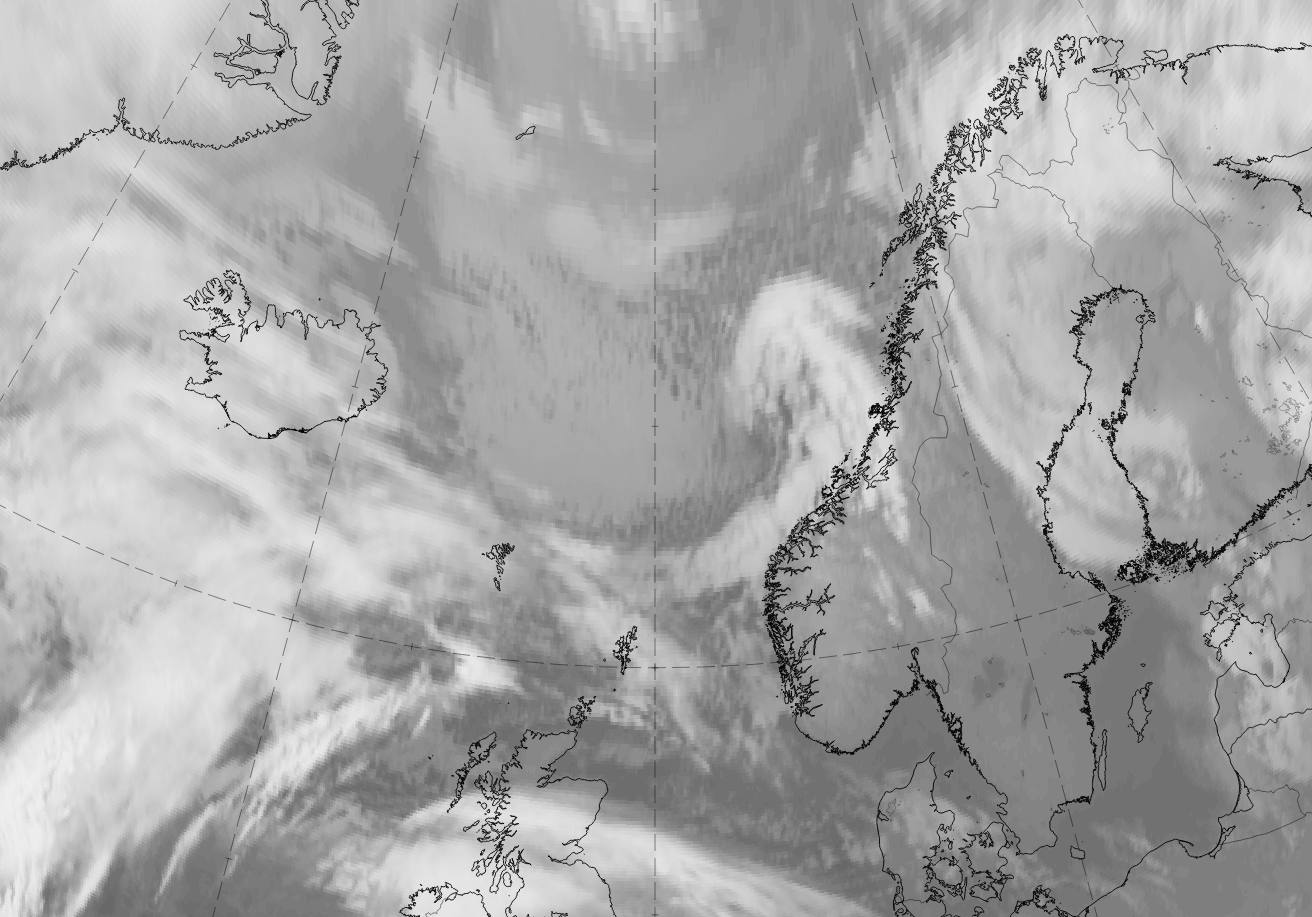
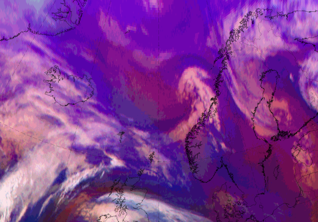
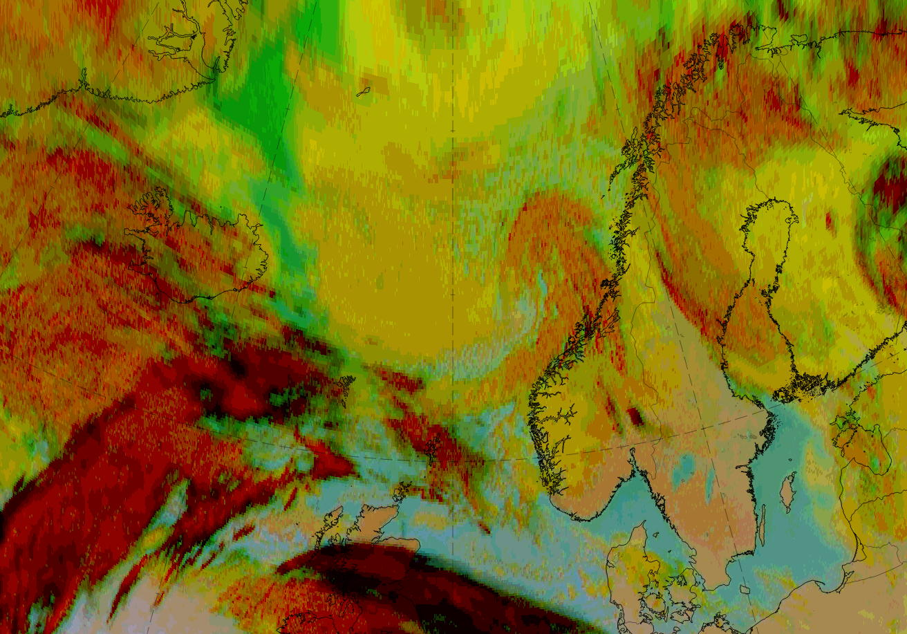
The case of 4 December 2018 can also be seen in the basic RGBs and compared among the basic channels and RGBs.
*Note: click on the image to access the image gallery (navigate using arrows on keyboard)
|
|
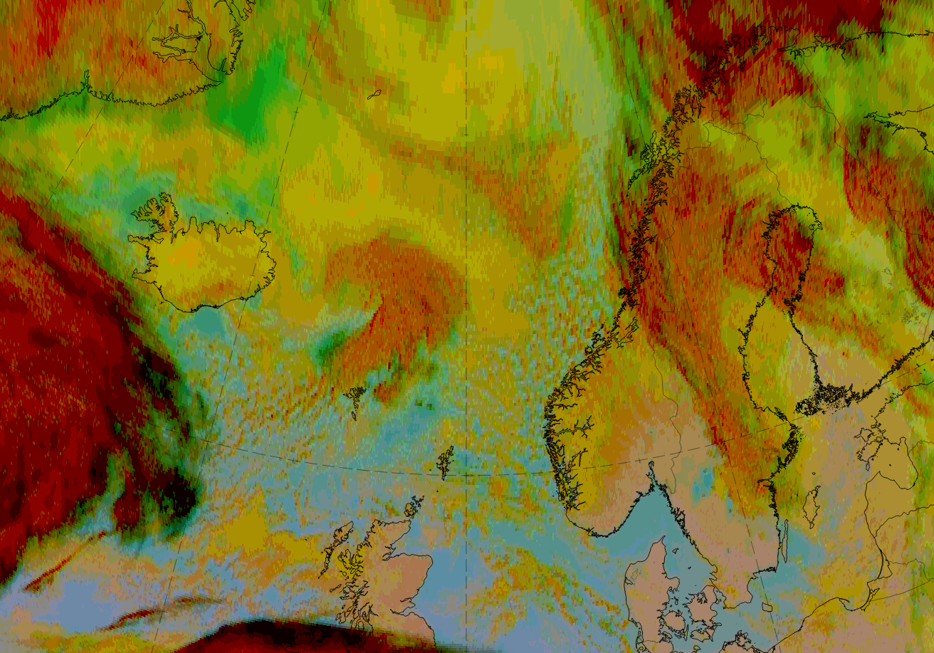
4 December 2018, 18UTC: 1st row: IR; 2nd row: WV (above) + Airmass RGB (below); 3rd row: Dust RGB + image gallery.
*Note: click on the image to access the image gallery (navigate using arrows on keyboard).
*Note: click on the image to access the image gallery (navigate using arrows on keyboard)
|
|

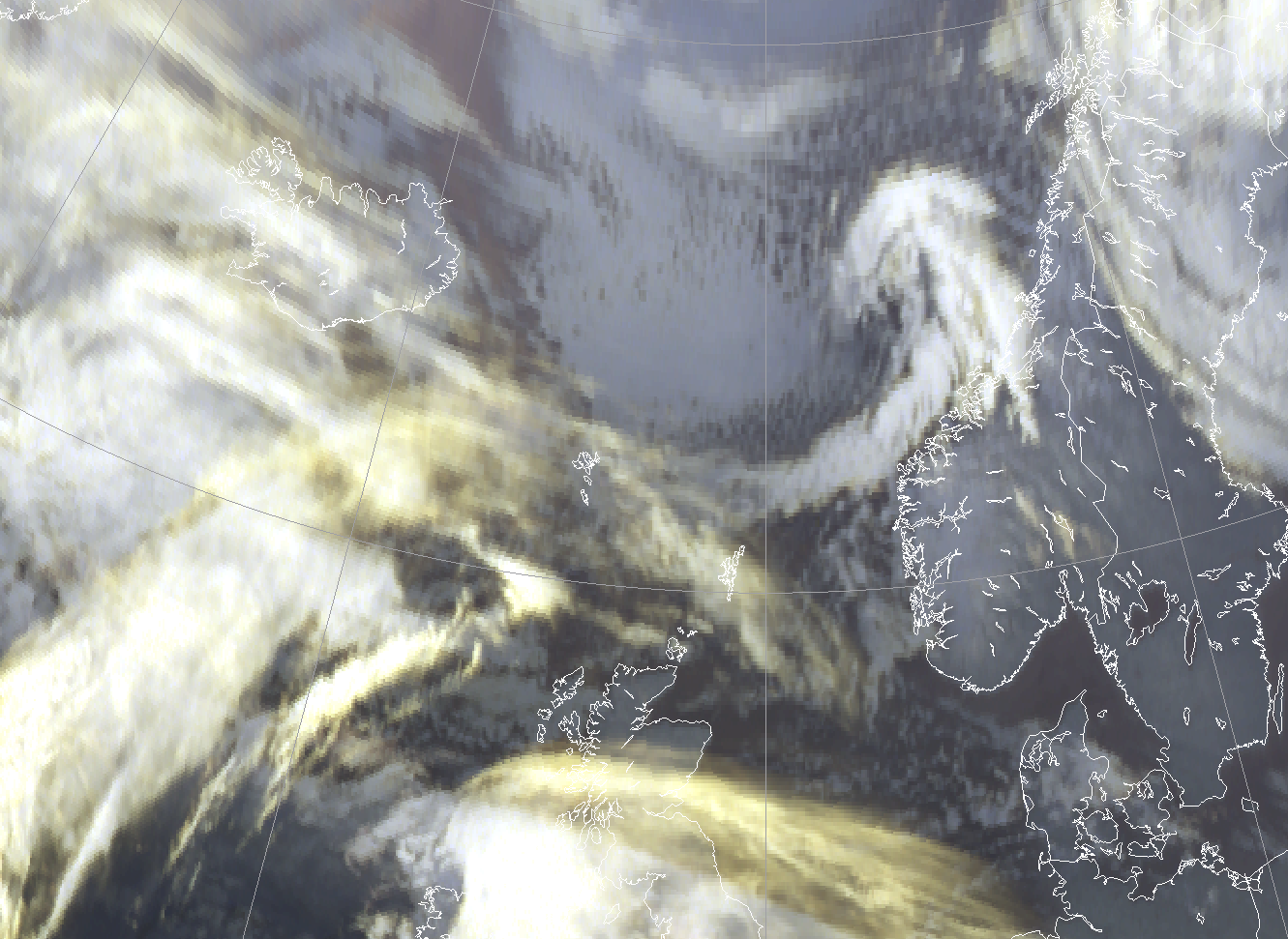
5 December 2018, 06UTC: 1st row: IR; 2nd row: WV (above) + Airmass RGB (below); 3rd row: Dust RGB + image gallery.
*Note: click on the image to access the image gallery (navigate using arrows on keyboard)
The two points of time representing the fully developed and the mature stage show very similar features in the basic channels and RGBs.
| IR | Distinct white comma spiral; innermost part of the comma head is light grey, representing warmer temperatures. |
| HRV | No visible channel available in this geographical latitude and at this time of year and day. |
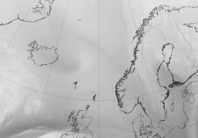
| WV | Cloud features are light grey; behind the polar low there is a dark grey area to the west. Northwest to the rearward edge of the comma spiral there is sinking stratospheric air. |
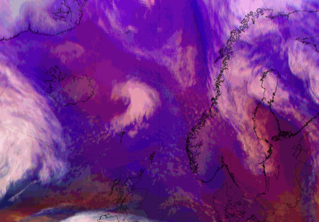
| Airmass RGB | Comma cloud embedded within dark blue colours representing the cold air behind the polar front. A dark red area behind the comma extends from the northwest to the rear edge of the comma spiral and represents the stratospheric, drier air. The comma cloud is overlaid by the dry air, hence the (usually white) clouds appear to have reddish colours. |
| Dust RGB | The comma feature is light red to brown, representing thick ice cloud but with lower cloud tops, as expected in thick comma features. Ochre colours around the comma cloud represent low to mid-level cloud, green colours represent mid-level cloud. |
Other sources of satellite imagery of Polar Lows
As polar lows normally form over the vast sea areas at high latitudes, the are few synoptic observations available. However, there are several types of satellite instruments that measure wind at the sea surface based on the back-scattering of active radar. The back-scatter is affected by the capillary waves at the surface, which is directly dependent on wind speed (and direction). Such measurements are known to be heavily contaminated by rain, but less so by snow, and hence they are quite useful to study Polar Lows.
ASCAT
The ASCAT and previously the Quickscat is the currently main source of information of wind over sea, and when combined with ordinary IR satellite imagery, gives excellent information. As of 2018, the resolution is 12,5km. The ascat gives information on wind speed and direction. An artifact of the instrument design is that the wind direction have three possible solutions, and the best guess based on a model input from the ECMWF-HIRES is selected. In a Polar Low where there are very sharp gradients in speed and direction, the model guess is not always correct, so errors in direction is common, but this is of less importance since a correct guess of the direction can be made by comparing with an IR-satellite image or simply considering the known and quite predictable wind pattern around a Polar Low.
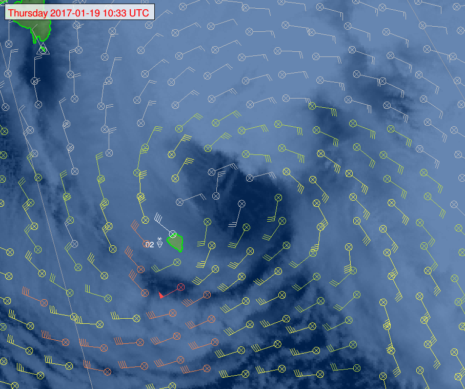
Figure 1.11: A close-up of ASCAT winds combined with an IR AVHRR satellite image with is made 50% opaque shows storm force winds southwest of the center of the low. Also the synoptic from Bear Island (white) is included in this composite. Illustration: MET-Norway/NOAA/Eumetsat
SAR
Syntetic aperture radar e.g. from the Sentinel 1 has a resolution of 5x20m and as such gives a very detailed impression of the wind pattern at the sea surface. Currently the images cover quite small areas (20x20 km), at intermittent intervals of 100 km along the path. In earlier years the regularity were such that these were not part of the operational basis of observations, but this has been improve with the launch of the Sentinel 1. The SAR images are most useful for studying the finer details, e.g. the shear zones associated with polar lows.
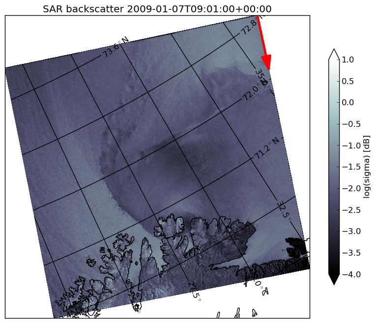
Figure 1.12: A rare SAR image capturing a polar low as it makes landfall at the coast of eastern Finnmark. Illustration: Furevik/MET-Norway
Bright colors in Figure 1.12 indicate strong winds. Dark is light winds. The shear zone between the western windy side and the eastern more quiet side is about 1 km wide, which explains why this is such a feared phenomenon in the coastal communities. The center of the low appears as dark, indicating that there are deceptively light winds here. The image also show that there is a smooth and focused flow around the center of a mature polar low, as opposed to the more disorganized flow in e.g. a cluster of Cb or a decaying polar low.