Table of Contents
Cloud Structure In Satellite Images
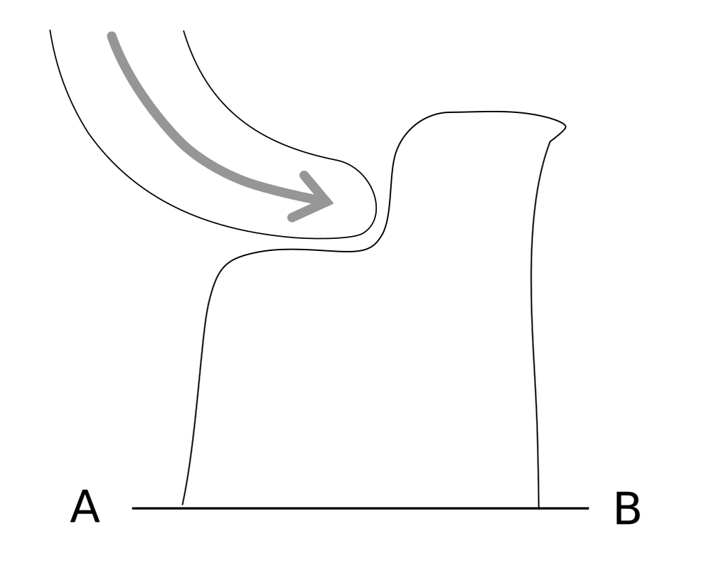
Definition: A Split Front is accompanied by a cyclonically curved cloud band, which, contrary to a classical Cold Front (see Cold Front ), contains a distinct double banded structure with cold cloud-top temperatures at the leading edge and warmer cloud-top temperatures at the rear edge.
Appearance in the basic channels
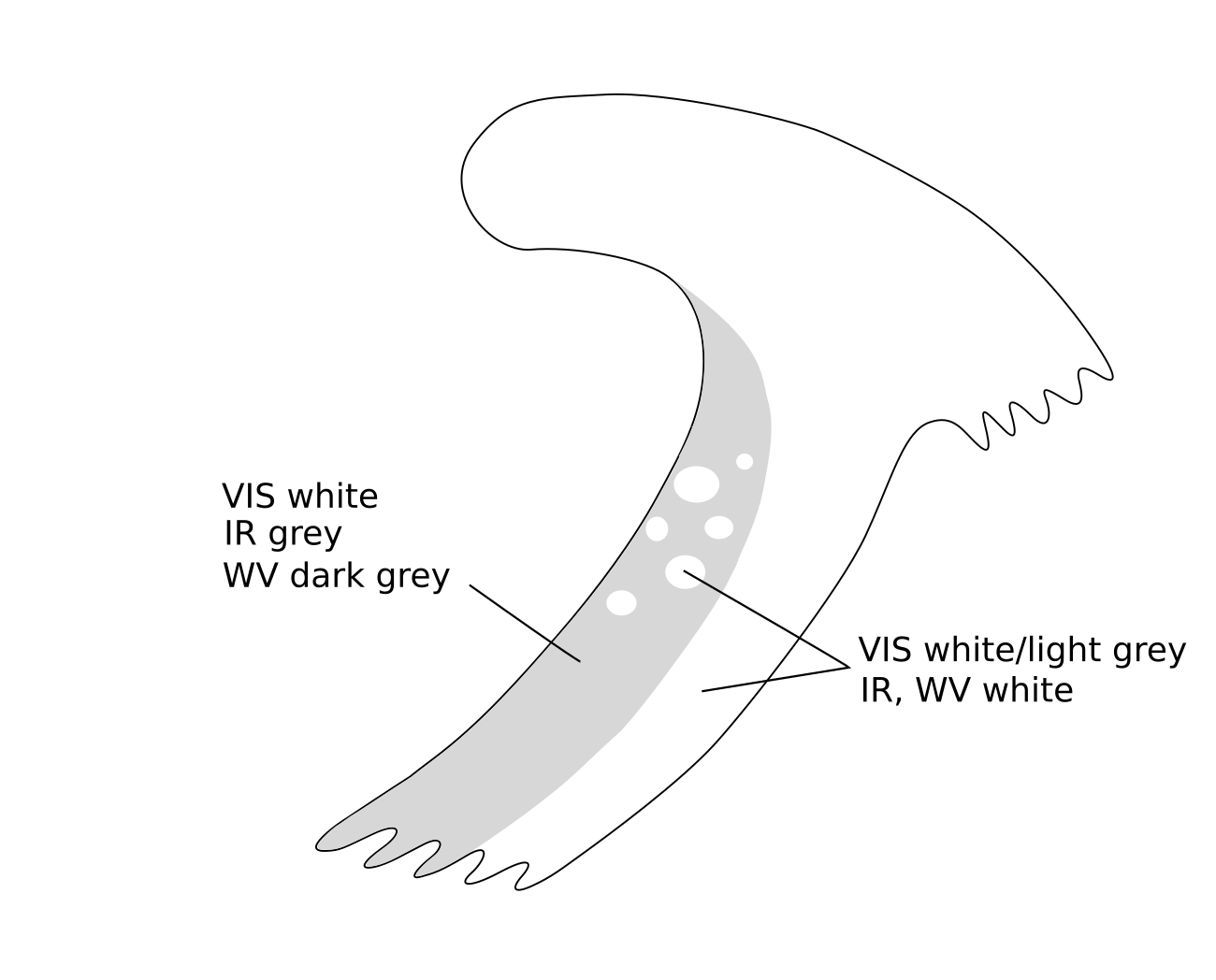
- In the thick cloud band at the leading part of the Split Front, VIS signals are white to grey and IR and WV signals are white, representing a thick, multi-layered cloud band
- In the low cloud band at the rear part of the Split Front, VIS signals are white and IR signals are dark grey to grey, WV signals are either black (if one is using the Meteosat 8 WV 6.2 µm , which shows higher level water vapour) indicating a low cloud band with very dry air above, or are fairly white/light grey if the Meteosat 8 WV 7.3 µm representing the lower atmosphere is used
- In the ideal case the boundary between both cloud bands is marked by a sharp gradient of IR and WV pixel values. In reality only a gradual change of IR and WV grey shading exists
- Some features of a life cycle can be observed:
- often EC shaped cellular clouds develops within and above the low cloud band on the cyclonic side of the jet axis;
- in the WV imagery a black area sometimes develops on the anticyclonic part of the jet axis over the low cloud band of the front, indicating sinking dry air connected with relative streams (see Meteorological physical background);
- in a multi-layered leading cloud band the higher cloud fibres are shifted downstream and the high and low cloud bands become decoupled.
Note: In the literature (especially in the US) the name split front has been used in relation to an upper-level Cold Front. This is comparable to "frontal delay by mountains" and "decoupling of cloud layers at different heights" in this manual (see Orographic Effects on Frontal Cloud ).
 |
 |
 |
Appearance in the basic RGBs:
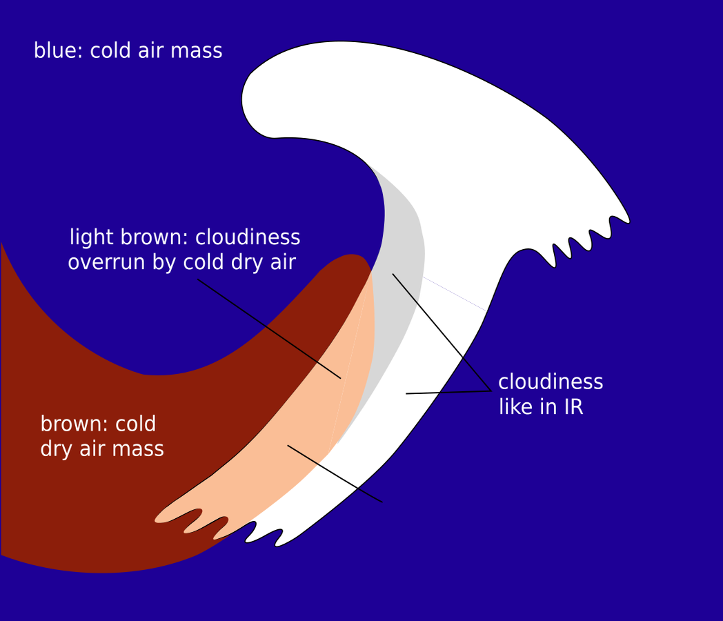
Airmass RGB
In the Airmass RGB there are usually blue to brown colours ahead of the split front, representing the airmasses in the upper-level trough area of the preceding frontal system. At the rear side there are blue and brownish colours representing the cold and dry air sinking from high latitudes and high altitudes towards the cloud bands of the split front. Contrary to most conceptual frontal models, the dark-brown stream overruns the lower cloud band of the split front.
While the lower cloud band at the rear of the split front has brownish colours, the higher cloud band at the leading side of the split front appears very similarly to that seen in the IR image.
Dust RGB
In the Dust RGB there are blue to pinkish-blue colours on both sides of the cloud band of the split front where there are cloud free areas; other existing, mostly mesoscale, cloud systems appear in ochre colours representing low to mid-level cloud.
The split characteristics of the cloud band belonging to a split front is also the main characteristic in the dust RGB. The lower cloud part at the rear of the system has mainly ochre colours indicating mid-level cloud tops, while the higher cloud part at the leading edge of the system has dark-red colours indicating thick ice clouds. Black fibres can also occur, mostly at the leading cloud edge, representing high translucent cloud fibres. Within the lower cloud part at the rear side, meso scale areas consisting of small dark-red cells can appear. They are connected to the peak of the cyclonic vorticity advection in the left exit region of the crossing jet streak (see Meteorological physical background).
 |
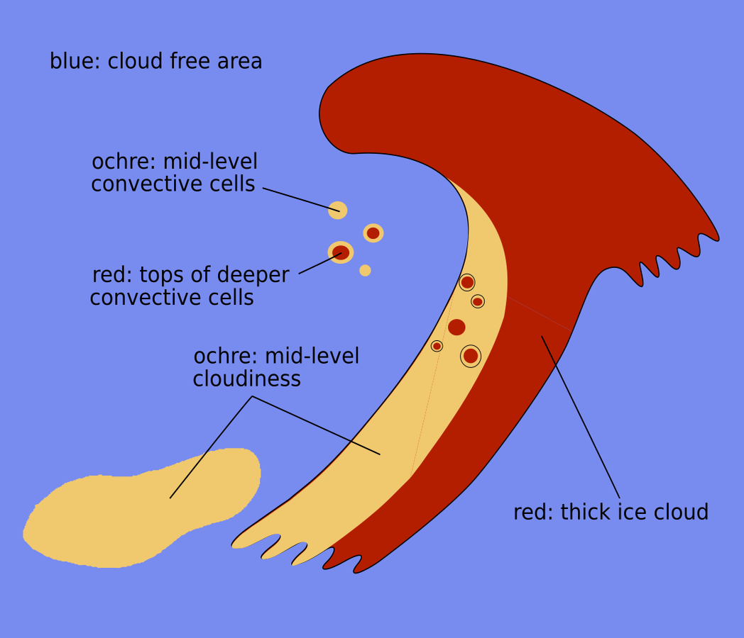 |
Legend: Basic RGBs schematics. Left: Airmass RGB; right: Dust RGB.
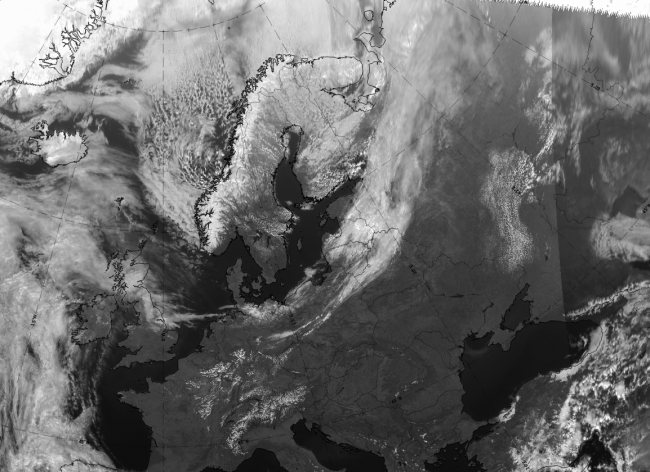
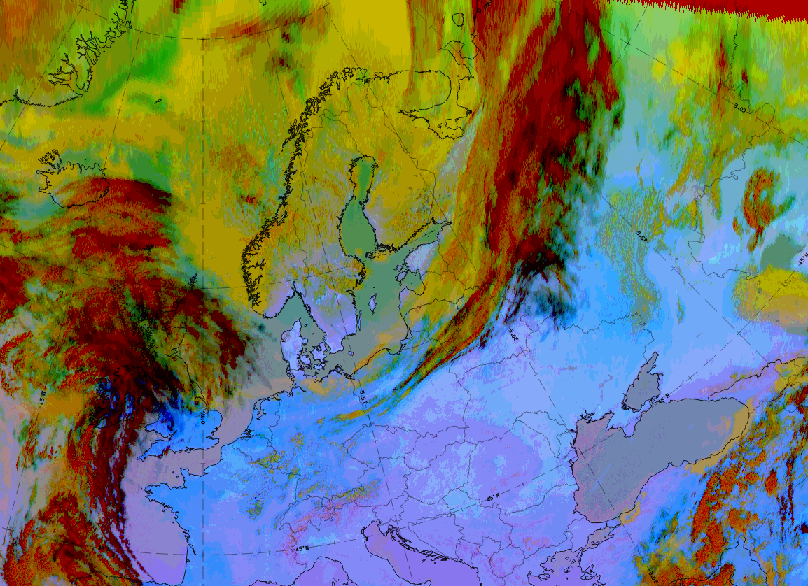
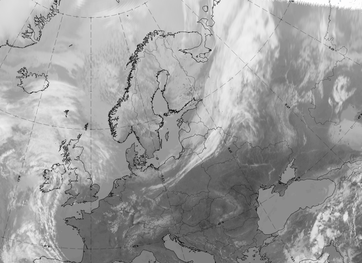
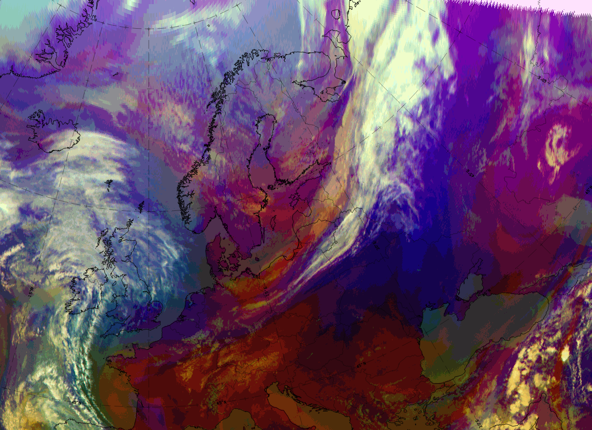
The case of 9 April 2020 at 12 UTC is a good example over Northeast Europe. It shows the double structure of the two cloud parts and the overrunning of dry air over the rearward lower cloud part.
|
|

|
|


Legend:
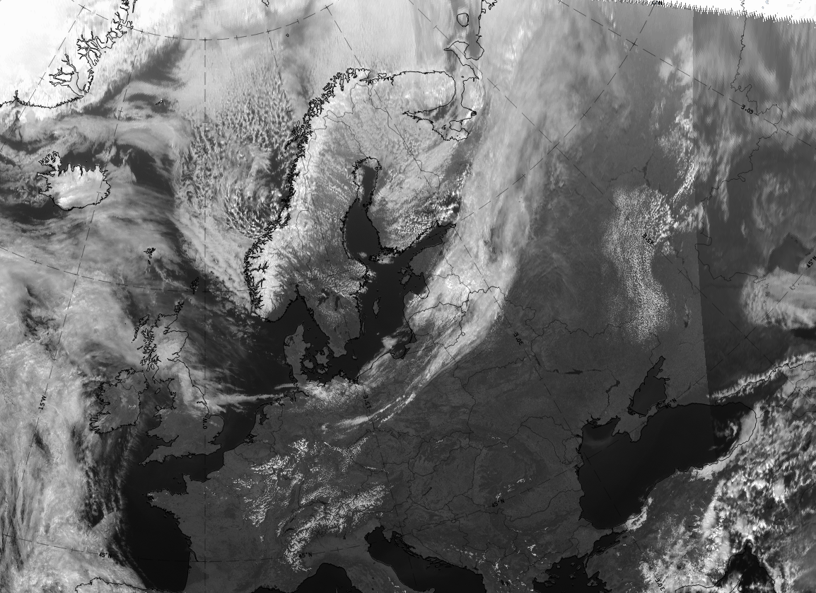
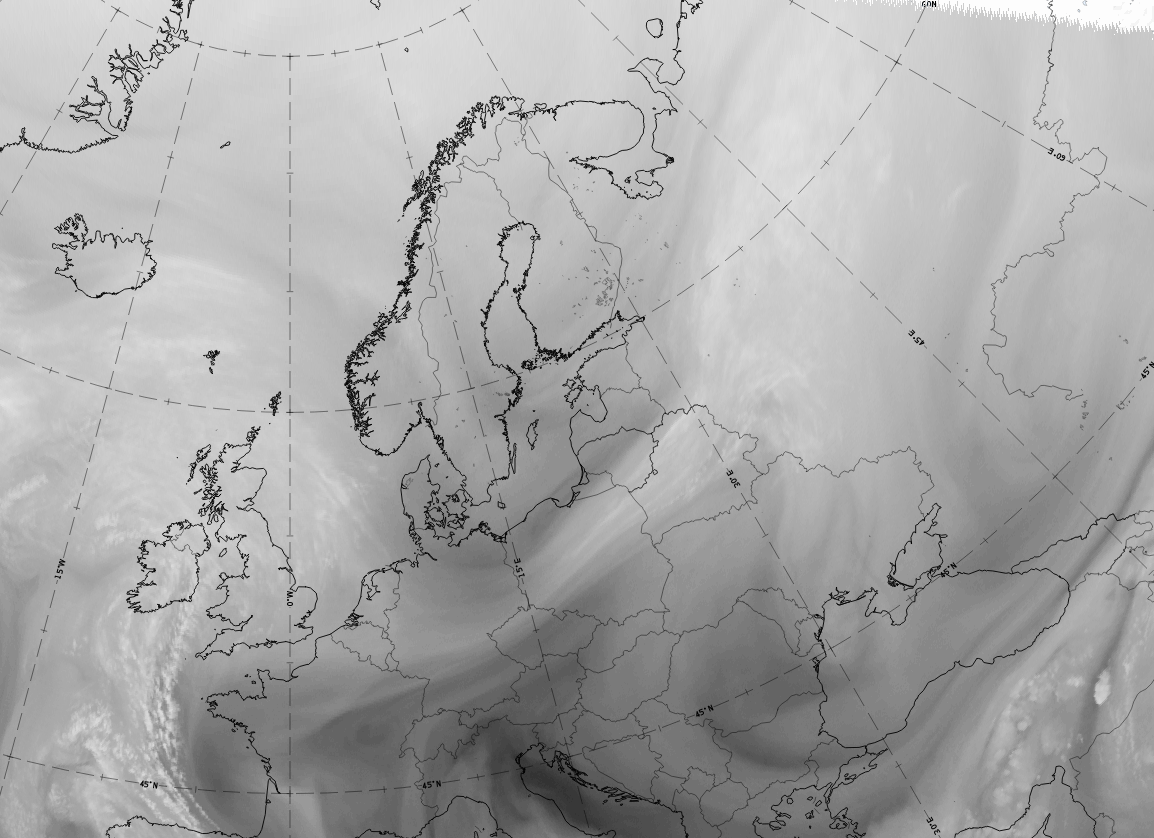
9 April 2020, 12UTC: 1st row: IR (above) + HRV (below); 2nd row: WV (above) + Airmass RGB (below); 3rd row: Dust RGB + image gallery.
*Note: click on the image to access the image gallery (navigate using arrows on keyboard).
| IR | White cloud band at the leading side, grey cloud band at the rear side, representing the two different high cloud parts of the split front. |
| HRV | White to light grey for large parts of both cloud bands. |
| WV | Black stripe along the coastal areas of the Baltic sea and across the Baltic states. This is above the lower cloud part of the split front and represents the sinking, dry air that is responsible for the dissolution of higher clouds. Light grey to white shading in the east, above the higher part of the split front. |
| Airmass RGB | Dark-brown stripe above the lower part of the split front indicating the sinking, dry air which is responsible for the dissolution of the higher cloud tops. Clouds of the higher part of the split front are similar to the IR image. Around the system dark -blue to dark-brown colours indicate the cold and dry air. |
| Dust RGB | Ochre to light-brown colours accompany the lower part of the split front, dark-red colours the thicker part. Some black stripes representing thin ice clouds can be found at the leading eastern and southern part of the split front. The surrounding areas of the split front are mostly blue-coloured, indicating cloud-free ground. |
The area within the lower cloud band in the split front, where thick convective cells are connected to a peak of cyclonic vorticity advection, cannot be seen in every case. The following case of 24 May 2020 shows at 15 UTC such a centre of enhanced cells, which corresponds to the left exit region of a crossing jet streak (enhanced by curvature vorticity in the trough) with a peak of cyclonic vorticity advection there.
Legend: 24 May 2020, 15 UTC
Left: Dust RGB: Right: IR, yellow: isotachs at 250 hPa; red: Cyclonic vorticity advection at 250 hPa.
*Note: click on the image to access the image gallery (navigate using arrows on keyboard).
Meteorological Physical Background
The conceptual model of a Split Front is strongly associated with jet streaks and sinking of very dry stratospheric air.
The initial stage of a Split Front is generally an Ana Cold Front type (see Cold Front - Meteorological physical background ). In contrast to the Ana Cold Front, the Warm Conveyor Belt is overrun aloft by the relative stream of the dry intrusion (the Conveyor belt theory). This process takes place as the warm air ascends ahead of the surface cold front with a forward component relative to the frontal system.
Looking at the situation on isentropic surfaces, the meteorological process which leads to the typical appearance of a Split Front in the satellite images can be explained as follows: together with a jet streak approaching the frontal cloud band, dry stratospheric air is advected on the cyclonic side, and dry tropospheric air on the anticyclonic side of the jet axis. Both air streams are sinking at this stage of development. Relative streams on the isentropic surface are parallel to the jet axis within the jet streak but show a characteristic splitting in the exit region into a northwards oriented and a southwards oriented component. While the southern branch is still sinking, the northern branch is rising again. During an interaction of jet streak and frontal cloud band this configuration of relative streams causes dissolution of cloudiness from above and the Split Front character then appears.
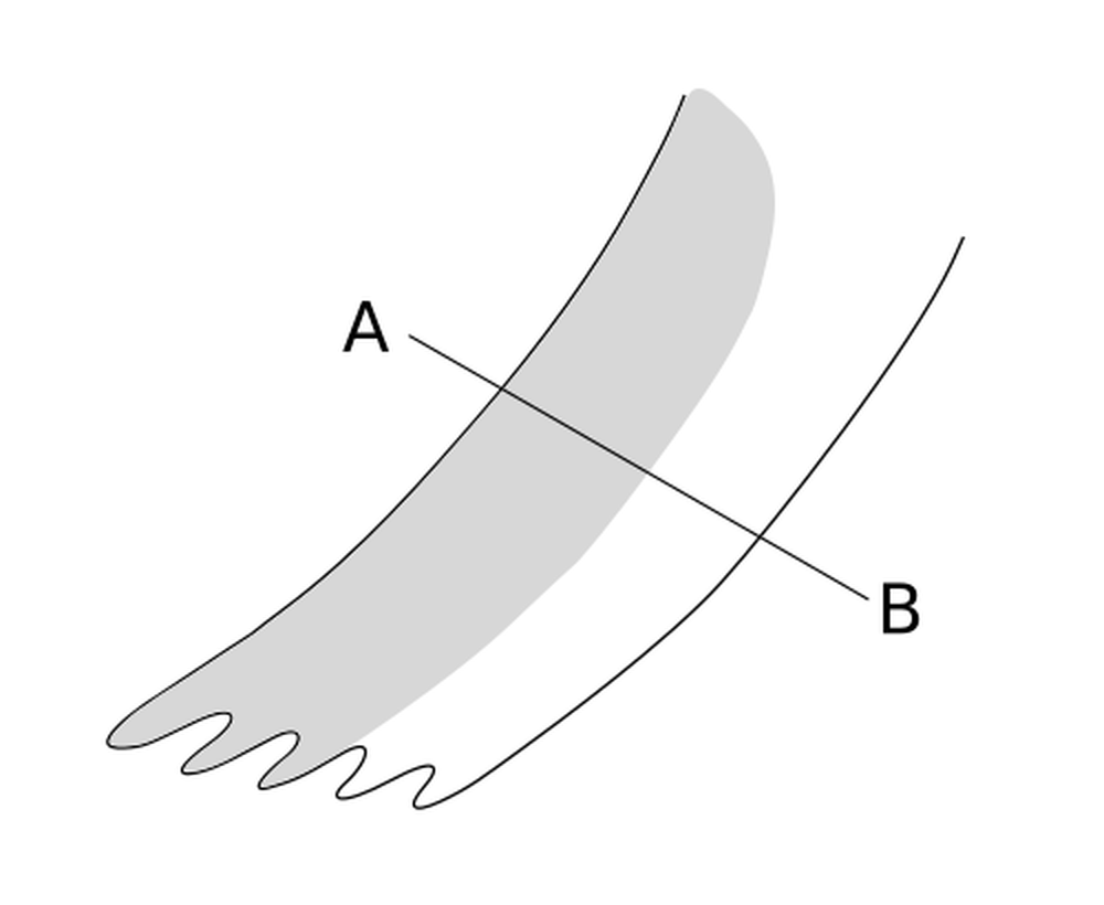
One way to classify the rear edge of the low cloud band is to regard it as a surface front and the rear edge of the high cloud band as an upper level front (see Cloud structure in satellite image). Between these frontal surfaces a shallow moist zone remains (see Weather events). A characteristic feature of the upper level front is that this frontal surface is a moisture boundary and not a thermal boundary (see Typical appearance in vertical cross sections).
Associated with the approaching jet streak, a PVA maximum situated in the left exit region may be superimposed upon the low cloud band of the Split Front ( link to Jet Streak model). Within this area the development of the above mentioned EC-like cloudiness can often be observed (see Front Intensification By Jet Crossing - Cloud structure in satellite image ).
|
|
30 August 2005/06.00 UTC - Meteosat 8 IR 10.8 image; magenta: relative streams 318K - system velocity 236°15 m/s, yellow: isobars 318K,
position of vertical cross section indicated
|
30 August 2005/06.00 UTC - Vertical cross section; black: isentropes (ThetaE), blue: relative humidity, orange
thin: IR pixel values, orange thick: WV pixel values
|
|
|
Looking at the vertical cross section, the humidity maximum in front and above the 318K surface between 500 and 350 hPa represents the warm conveyor belt (accompanied by peaks in IR and WV pixel values) while on this isentropic surface further upstream, near 350 hPa one can see drier air, which is connected to the relative streams bringing dry stratospheric air over the frontal region.
Key Parameters
- Temperature advection (WA):
The ridge of WA is superimposed on the high level cloudiness representing the warm air rising on the upper level frontal surface. - Jet streak and positive vorticity advection (PVA):
A jet streak approaches the cloud band at a large acute angle accompanied by a PVA maximum in the left exit region. - Humidity:
Very dry values in the upper and middle troposphere above the low level cloud band and a strong gradient between the two cloud bands at different heights can be observed. - Relative streams and potential vorticity (PV):
Typical configuration of relative streams as described in the Meteorological physical background, PV anomaly on relevant isentropic surfaces indicating stratospheric air.
|
30 August 2005/06.00 UTC - Meteosat 8 IR 10.8 image; red: positive vorticity advection (PVA) 300 hPa, yellow:
isotachs 300 hPa
|
|
|
|
Typical Appearance In Vertical Cross Sections
In the ideal case the isentropes of the equivalent potential temperature show two frontal gradient zones, an upper level front and a surface front. Both zones have Cold Front inclinations. While the upper level front is connected to the high leading cloud band, the surface front represents the low-level cloudiness to the rear of the frontal system. Whereas the zone of the surface front is pronounced, that of the upper level front is quite weak. Therefore, the upper level front is not characterized as a thermal boundary but rather as a moisture boundary (see Meteorological physical background).
The field of temperature advection often shows pronounced WA in front of and above the upper level frontal zone, which is connected with the upper level cloudiness. CA, typical for Cold Fronts, is situated below the surface front.
The most characteristic feature of the humidity distribution is a dry area at higher levels between the two frontal zones. High values of humidity can be found in front of the frontal zones.
In the case of superimposed EC cloudiness, a distinct isotach and PVA maximum can be found above the surface front at approximately 300 hPa (see Front Intensification By Jet Crossing - Typical appearance in vertical cross section ).
Looking at the distribution of humidity the satellite signals, IR and WV images show the highest pixel values in front of the upper level front and, if existing, within the EC - like cloud. To the rear of the upper level front the VIS signals are usually higher while IR and WV signals are much lower than those in front of the upper level front (see Cloud structure in satellite image).
Compare the chapter Cloud structure in satellite image, where the cross section is indicated in the image. In contrast to the ideal case the surface Cold Front has a superadiabatic layer in the lower levels of the troposphere. The upper level Cold Front is well developed. The distribution of humidity shows the described insertion of drier air between the two frontal zones. The IR and WV images show the pronounced decrease of temperature from the low to the high cloud part.
|
30 August 2005/06.00 UTC - Meteosat 8 IR 10.8 image; position of vertical cross section indicated
|
|
|
30 August 2005/06.00 UTC - Vertical cross section; black: isentropes (ThetaE), blue: relative humidity, orange
thin: IR pixel values, orange thick: WV pixel values
|
|
|

|
|
30 August 2005/06.00 UTC - Vertical cross section; black: isentropes (ThetaE), green thick: vorticity advection
- PVA, green thin: vorticity advection - NVA, orange thin: IR pixel values, orange thick: WV pixel values
|
|
|
|
|
30 August 2005/06.00 UTC - Vertical cross section; black: isentropes (ThetaE), yellow: isotachs, orange thin:
IR pixel values, orange thick: WV pixel values
|
|
|
|
Weather Events
Weather events are highly variable and have to be split into two parts: the upper level front and the shallow moist area.
Upper front
| Parameter | Description |
| Precipitation |
|
| Temperature |
|
| Wind (incl. gusts) |
|
| Other relevant information |
|
Shallow moist area, including the surface front
| Parameter | Description |
| Precipitation |
|
| Temperature |
|
| Wind (incl. gusts) |
|
| Other relevant information |
|
|
|
|
Legend:
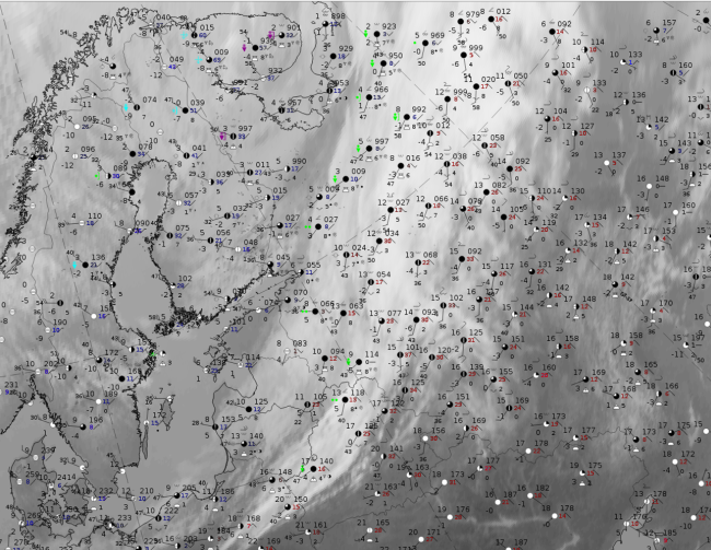
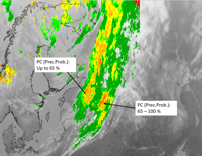
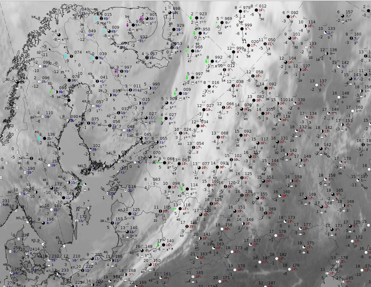
9 April 2020, 12UTC: IR + synoptic measurements (above) + probability of moderate rain (Precipitting clouds PC - NWCSAF).
Note: for a larger SYNOP image click this link.
There are many Cb and precipitation reports. In the thick part, on the leading side of the split front, a row of Cb observations with associated showers stretches from Belarus northward; they are close to the rearward edge of this thick cloud band. In the southern part of the low cloud band there are only overcast skies, located over the Baltic States, and some observations of persistent precipitation over Russia. More to the north, again thunderstorms and showers also exist. Those are connected to a maximum of cyclonic vorticity advection. The probability of precipitation computed from the PC product (NWCSAF) shows parallel, bandlike stripes with higher probabilities for both cloud bands.
|
|
|
|
Legend:
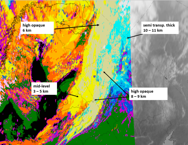
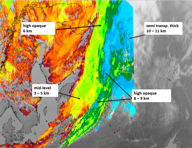
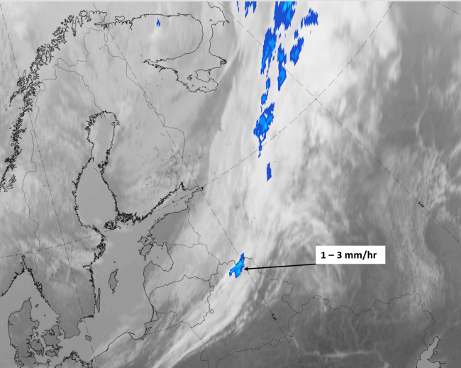
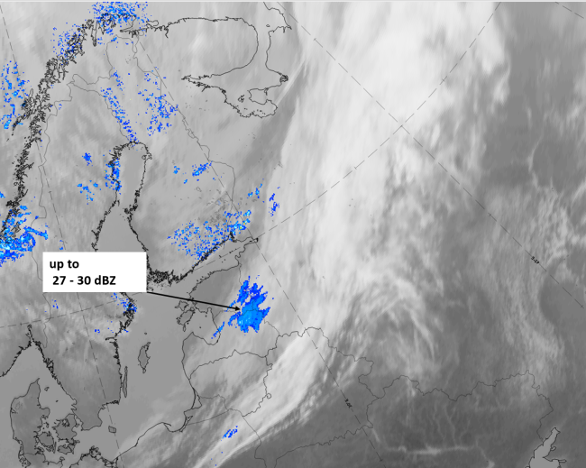
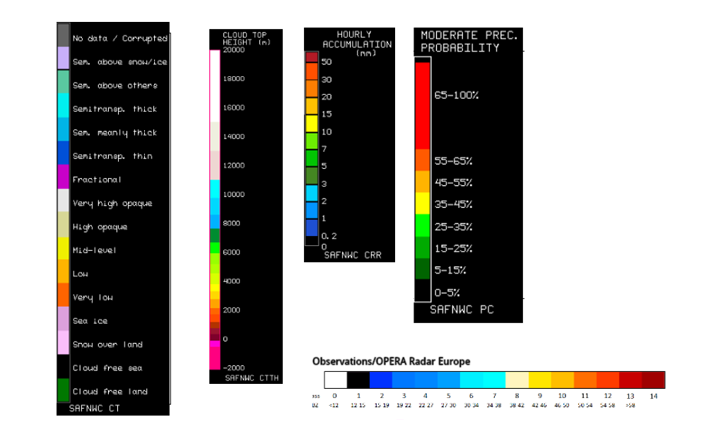
9 April 2019, 12 UTC, IR; superimposed:
1st row: Cloud Type (CT NWCSAF) (above) + Cloud Top Height (CTTH - NWCSAF) (below); 2nd row: Convective Rainfall Rate (CRR NWCSAF) (above) + Radar intensities from Opera radar system (below).
For identifying values for Cloud type (CT), Cloud type height (CTTH), precipitating clouds (PC), and Opera radar for any pixel in the images look into the legends. (link)
References
General Meteorology and Basics
- BROWNING K. A. (1985): Conceptual models of precipitation systems; Quart. J. R. Meteor. Soc., Vol. 114, p. 293 - 319
- BROWNING K. A. (1986): Conceptual models of precipitation systems; Weather&Forecasting, Vol. 1, p. 23 - 41
- CONWAY B. J., GERARD L., LABROUSSE J., LILJAS E., SENESI S., SUNDE J. and ZWATZ-MEISE V. (1996): COST78 Meteorology - Nowcasting, a survey of current knowledge, techniques and practice - Phase 1 report; Office for official publications of the European Communities
- GREEN J. S., LUDLAM F. H. and MCLVEEN J. F. R. (1966): Isentropic relative-flow analysis and the parcel theory; Quart. J. R. Meteor. Soc., Vol. 92, p. 210 - 219
- HUBER-POCK F. and KRESS CH. (1989): An operational model of objective frontal analysis based on ECMWF products; Met. Atmos. Phys., Vol. 40, p. 371 - 382
- KURZ M. (1990): Synoptische Meteorologie - Leitfäden für die Ausbildung im Deutschen Wetterdienst; 2. Auflage, Selbstverlag des Deutschen Wetterdienstes
- ZWATZ-MEISE V. (1987): Satellitenmeteorologie; Springer Verlag, Berlin - Heidelberg - New York - London - Paris - Tokyo
General Satellite Meteorology
- BADER M. J., FORBES G. S., GRANT J. R., LELLEY R. B. E. and WATERS A. J. (1995): Images in weather forecasting - A practical guide for interpreting satellite and radar imagery; Cambridge University Press
Specific Satellite Meteorology
- BROWNING K. A. and MONK G. A. (1982): A simple model for the synoptic analysis of cold fronts; Quart. J. R. Meteor. Soc., Vol. 108, p. 435 - 452
- BRENNAN M. J., LACKMANN G. M. and KOCH S. E.: An Analysis of the Impact of a Split-Front Rainband on Appalachian Cold-Air Damming. pages 712-731, Vol 18, No 5, Oct 2003.
- HOBBS P. V., LOCATELLI J. D. and MARTIN J. E., 1996: A new conceptual model for cyclones generated in the lee of the Rocky Mountains. Bull. Amer. Meteor. Soc., 77, 1169-1178, 1996.