Chapter III: Instructions on how to identify Atmospheric Rivers
1. Identify the moisture pattern of an AR
The first step in identifying ARs consists of looking for long and narrow bands of moisture with a column integrated liquid water content of more than 20 mm. For this, you can use satellite imagery and/or NWP diagnostic or forecast fields.
- ARs are moisture bands that are at least 2000 km long and less than 300 km wide
- They have a total column water equivalent of more than 20 mm
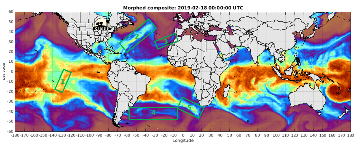
They can be best seen in microwave channels from polar orbiting satellites or in the Total Column Water (TCW) parameter from NWP models.
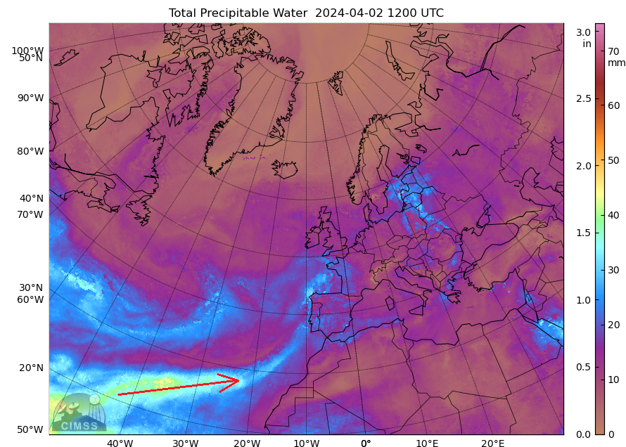
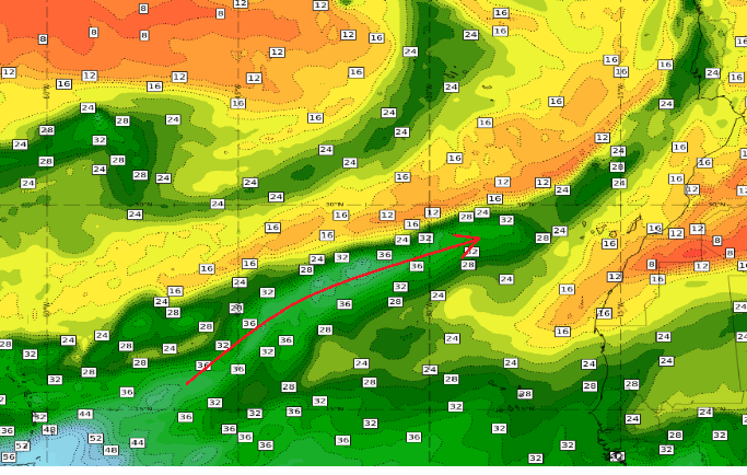
Figure 4: Left: MIMIC-TWP2 product (Microwave humidity sounder composite image), right: ECMWF Total Column Water [mm] from 2 April 2024 at 12:00 UTC. The red arrows depict the same moisture filament in the different projections.
Radiometer instruments are less suited to the detection of ARs, as most of the humidity is in gaseous form accompanied by only a few clouds. Water vapor absorption channels in the infrared spectrum currently do not show these low-level moisture features because of the missing sensitivity of the bands to low-level moisture. Warm water clouds within these moisture filaments show little optical contrast to the sea surface in the infrared image; the visible channels depict them better with the sea acting as a dark background (Figure 5). However, the Dust RGB has some ability to depict low-level moisture gradients in blue colour shades by using the split-window technique [BT10.8 − BT12.9].
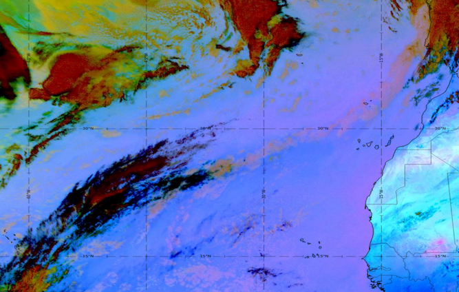
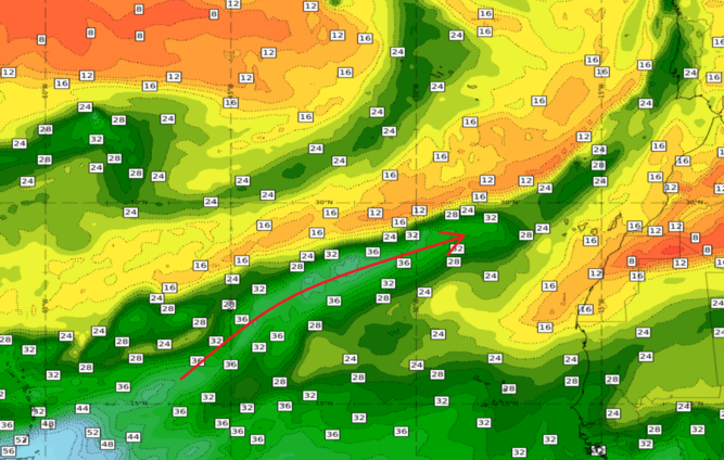
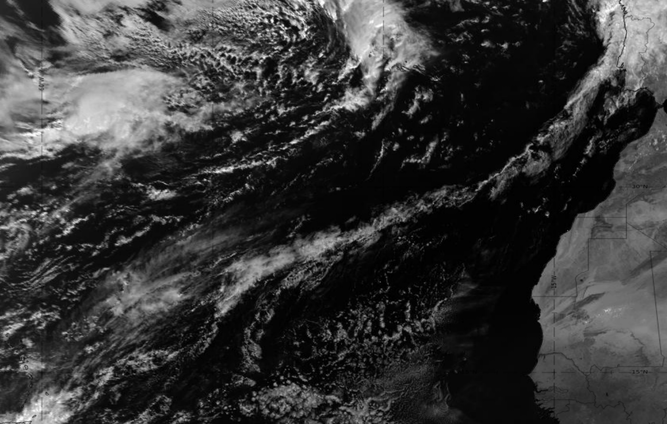
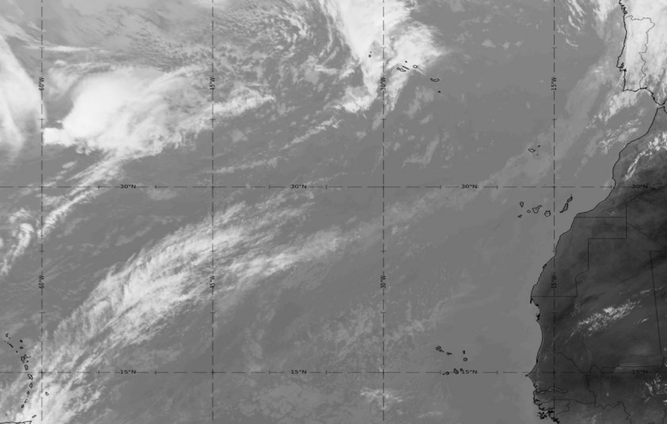
Figure 5: 2 April 2024, 12:00 UTC.
Top: SEVIRI Dust RGB and TCW from ECMWF. The red arrow depicts the moisture filament.
Bottom: VIS 0.8 μm and IR 10.8 μm SEVIRI images.
Once you have identified a moisture filament, it may not necessarily be an Atmospheric River; it could also be:
- a frontal zone (polar- or sub-tropical front)
- an air mass boundary
- an occlusion
- or a moisture convergence zone.
Hence, the next step to follow is to look at the vertical moisture distribution.
Exercise 1:
Identify potential candidates for ARs from the microwave satellite data and TCW model field.
2. Investigate the vertical moisture distribution
The next step consists of identifying the location of the moisture in the vertical profile.
The moisture in ARs is characterized by:
- high water vapour concentrations at layers below 700 hPa.
This characteristic of ARs is best analysed from model humidity fields.
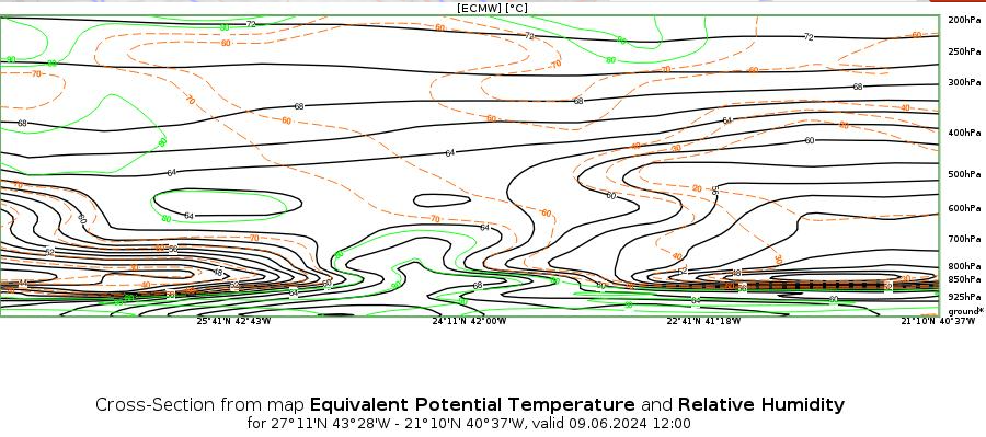
Figure 6: Vertical cross section through an AR. A bulge of high relative humidity values reaching up to 700 hPa
can be seen in the middle of the cross section.
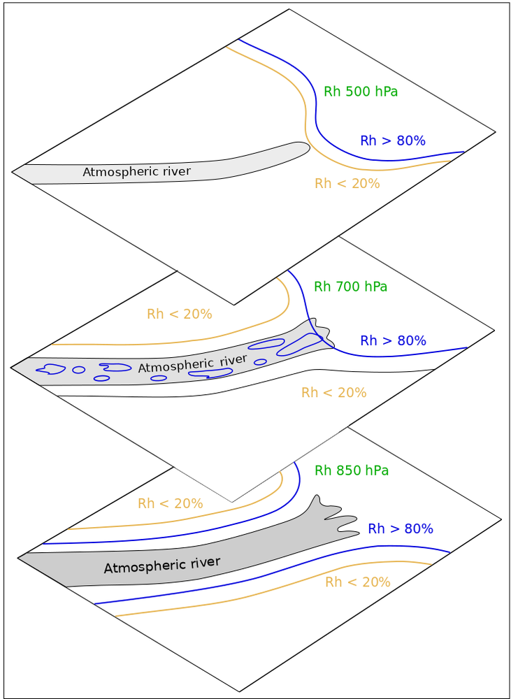
Figure 7: Left: 2-D charts of relative humidity at levels 500, 700 and 850 hPa. Right: Schematic of the relative humidity charts.
Most of all, "rivers in the sky" are characterized by their flow. In the next chapter, we find out how these moisture bands behave like rivers.
Exercise 2
Click on the images and go through the gallery, then answer the question.
Identify the model cross sections that show signs of an AR.
3. Identify the moisture transport
The third step consists of diagnosing the moisture transport. ARs are characterized by high moisture transport along the filament with:
- wind speeds at low levels (a.k.a. low-level jet) of more than 12.5 m/s.
A combination of high water vapor concentration (TCW > 20 mm) and wind speeds of more than 12.5 m/s within the AR results in a moisture transport of more than 250 kg m−1 s−1.
N.B.: 20 mm water = 20 kg m−2 ⟹ 20 kg m−2 * 12.5 m s−1 = 250 kg m−1 s−1
Low-level jets associated with these moisture bands are the result of pressure and/or temperature gradients along the AR. These pressure and temperature gradients are usually weak inside the tropical air mass from where they originate, but they usually become stronger as the AR moves north. However, many of these moisture outbreaks from tropical air masses do not meet favourable conditions to become an AR and dissolve.
When moisture filaments approach the cold front of a mid-latitude cyclone, temperature and pressure gradients usually increase in their vicinity and so does the low-level jet.
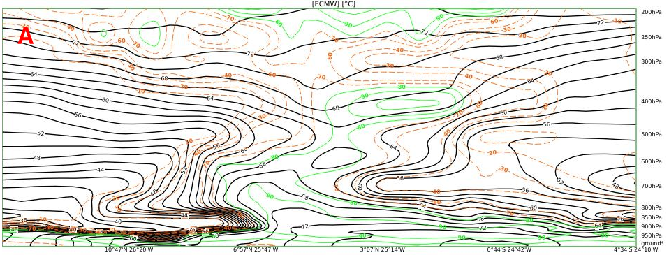
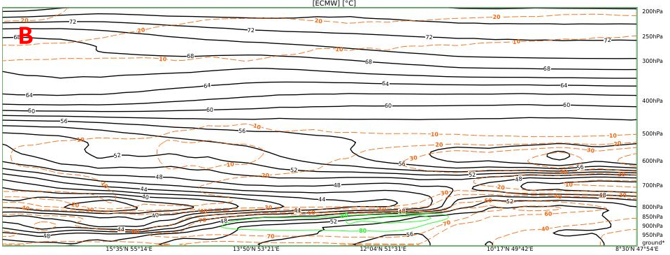
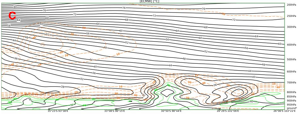
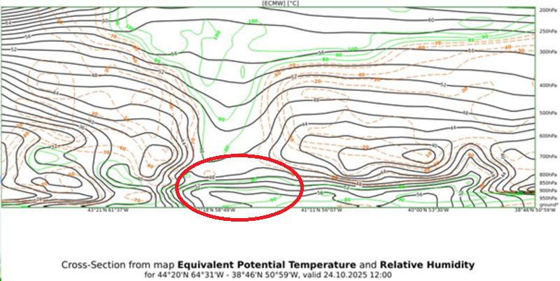
The wind profile in the cross section below shows a low-level jet accompanying the AR indicated by red cross (Figure 8).
Use the slider to compare the two images.
|
|
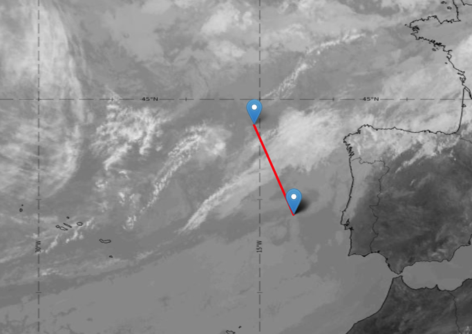
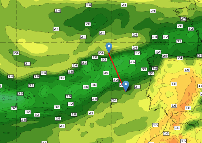
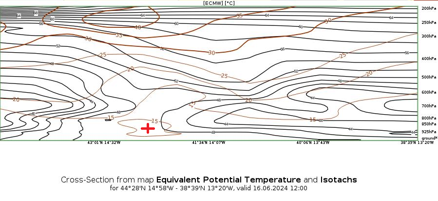
Figure 8: 16 June 2024 at 12:00 UTC.
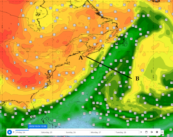
Top: SEVIRI IR10.8 and TCW from ECMWF. The red line indicates the position of the cross section.
Bottom: Equivalent potential temperature (black) and isotachs (brown) in the cross section through the AR.
After finishing step 3, ARs are detected. However, some ARs merge with cold fronts and then their characteristics are mixed with the features of the cold front.
In the next chapter, you will learn how to recognize ARs that have merged with a cold front.
Exercise 3:
Hover over the image to see the details.
Identify the low-level jet in the data sources provided:
4. Differentiate between frontal and non-frontal ARs
ARs originate from tropical marine air masses and are initially not connected to mid-latitude fronts. However, when moving to higher latitudes, they become attracted to the low-pressure systems of the polar front and often end up merging with a cold front.
So, how can we recognize an AR once it has merged with a cold front?
- The cold front shows high values of moisture in lower levels.
- A low-level jet can be identified.
- Winds run parallel to the surface front at lower levels below 700 hPa.
- The cold front is stationary or slowly advancing.
When ARs merge with a cold front, they usually find advantageous conditions such as pre-frontal convergence at lower levels, which increases the water vapour concentration, and stronger temperature and pressure gradients, which increase the low-level jet and the humidity transport.
The difficulty in discerning an AR merged with a cold front comes from the fact that cold fronts typically show high humidity values and stronger winds anyway. However, the characteristics of the AR should be preserved within the lower frontal zone. In such a case we can discern:
- high water vapor content below 700 hPa
- a wind speed maximum or at least an area with higher wind speed below 700 hPa
- a wind direction parallel to the front.
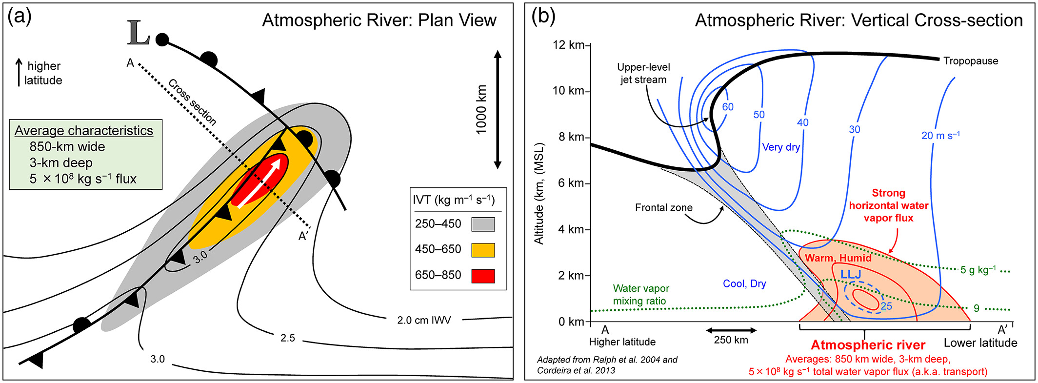
Figure 9: Left: Schematic of Integrated water Vapor Transport (IVT)
Right: Schematic of vertical moisture distribution and the low-level jet (LLJ), © Ralph et al., 2020.
Rapidly progressing cold fronts usually do not preserve the characteristics of an AR as in such a case surface winds tend to be perpendicular to the front, even at lower levels. These types of cold fronts can bring intense winds and heavy showers, but the duration is rather short so that the total amount of precipitation is not very high.
In the next chapter, we will see the impact of an AR when it makes landfall.
Exercise 4:
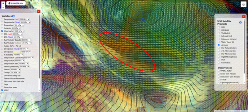
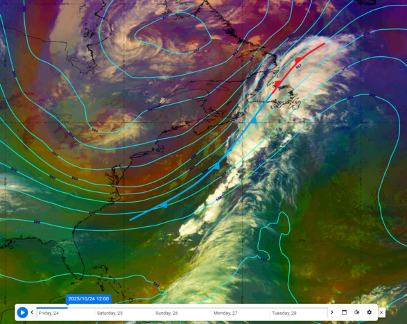
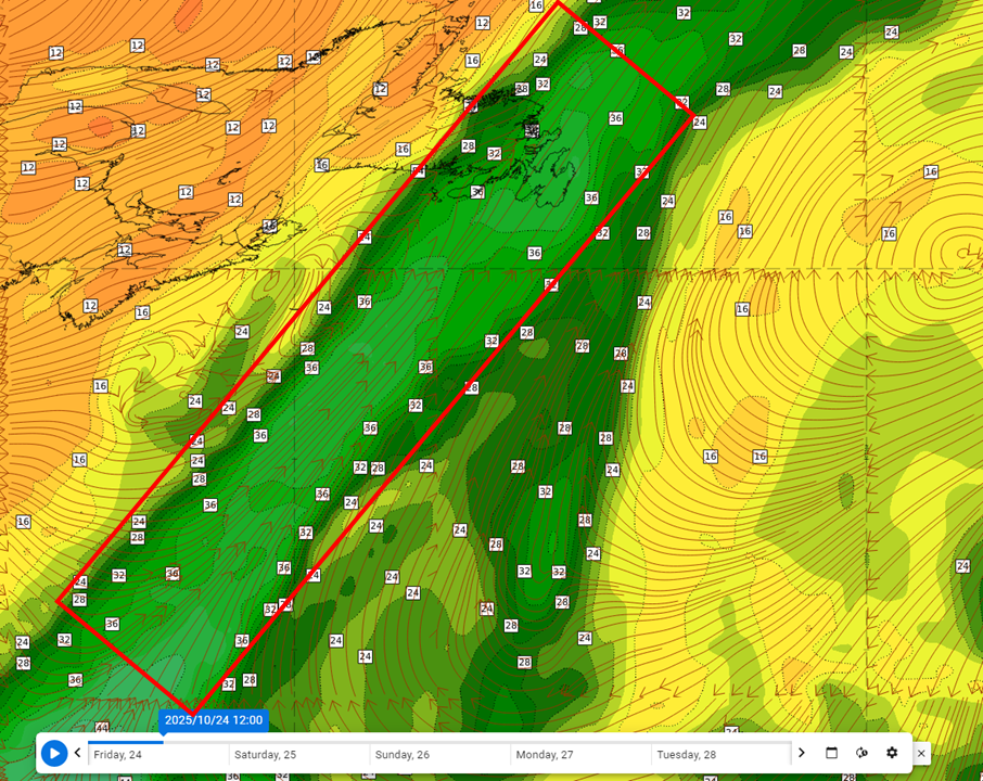
Look at the synoptic situation shown in the Airmass RGB below. You will see a cold front over the Atlantic and high Total Column Water values ahead of it.
Is there an AR merged with the cold front?
|
|
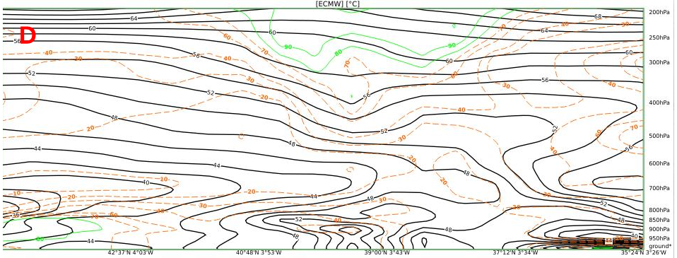
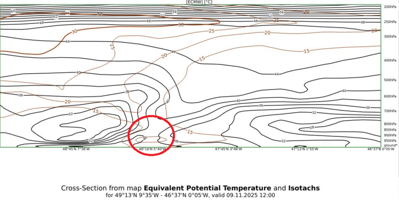
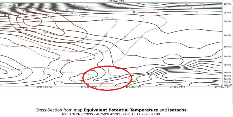
Let's start by identifying the cold front in the cross section. Draw the cold front:
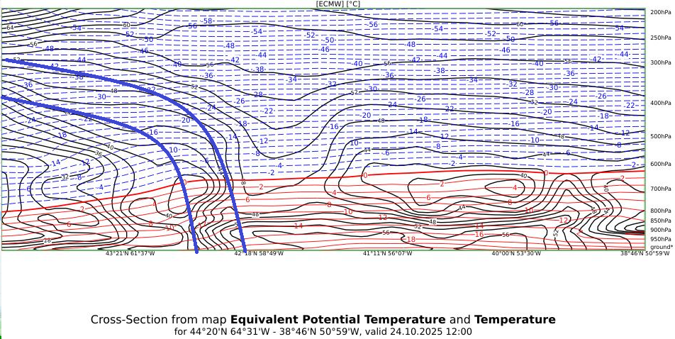
The next step consists of finding the high water vapor amounts ahead of the cold front at lower levels. Circle the AR:
Now let's check the presence of a low-level jet. Circle the low-level jet.

Now you have seen the most important features of a merged AR in the vertical cross section. However, we still have to confirm that the low-level jet runs parallel to the cold front.
As you can see in the image below, the streamlines at 925 hPa do indeed run parallel to the cold front (red box):
5. Evaluate the impact of an AR landfall
ARs are known to be the cause of abundant rainfall and flooding over mid-latitude coastal landmasses [4]. Preconditions for high precipitation rates over land are:
- strong moisture transport within the AR
- the AR being lifted over elevated orography
- the AR being stationary over a long time span.
When making landfall, higher wind speeds are expected over coastal water and the shore. Over land, friction reduces the wind speed at lower levels. Moreover, there seems to be a higher occurrence and impact of ARs in the winter season in the UK and western continental Europe [3][4].
Water vapor is released as precipitation when the AR is lifted over a mountain chain or over coastal elevation (Figure 10).
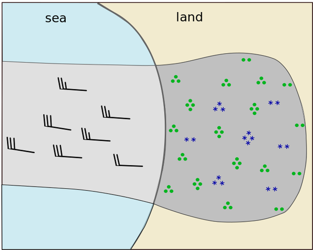
Figure 10:Schematic showing where precipitation occurs after an AR makes landfall.
Another important factor is the duration of the event. Most ARs hitting land in mid-latitudes are embedded in the cold front of a depression. Precipitation amounts are highest when the front is stationary and the wind is blowing in parallel to the front line. Much of the impact depends on the soil type, relief and population density.
We observe more ARs in the winter season [2][3], when cold air troughs extend more frequently to lower (tropical) latitudes (Figure 11) and then bring warm, moist air masses towards the poles.
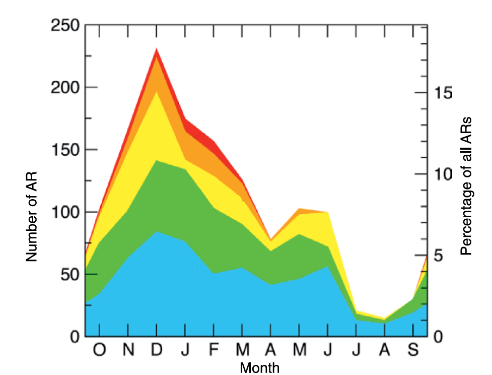
Figure 11: Seasonality of AR events near Bodega Bay (California) based on events from MERRA from January 1980 to April 2017, © Ralph et al., 2019.