Exercise: Po Valley Air Pollution Event in February 2019
As introduced in the previous section, the Po Valley is prone to frequent pollution episodes, especially during winter. For this exercise, the pollution episode of February 2019 has been selected to help learn how to interpret and combine information from several online resources.
On 19 February 2019, the Italian Regional Agency for Prevention, Environment and Energy of Emilia-Romagna (ARPAE) announced a smog alert. ARPAE reported a widespread increase in PM10 concentrations from 13 and 14 February onwards, which led to regulatory threshold (50 µg m-3) exceedance in almost the entire region from 15 to 17 February. High PM10 concentrations above the limit were recorded until Wednesday 20 February (highest values recorded are: 112 µg m-3 in Ferrara and 95 µg m-3 in Modena; ARPAE, 2019a).
From 22 to 25 February, emergency measures were taken in the municipalities belonging to the 'Air quality Plan' (PAIR) of the Emilia-Romagna region. These emergency measures, planned at the regional level, included the extension of traffic restrictions to vehicles with DIESEL EURO 4 and below. The traffic restrictions in urban centres for the most polluting vehicles remained valid every day (including Saturdays and Sundays) from 8.30 am to 6.30 pm (ARPAE, 2019b).
The reported levels of PM10 and nitrogen dioxide, could have caused minor health effects (such as irritated airways, coughing, and exacerbation of symptoms of an existing lung condition). Levels of other air pollutants were presumably also higher, as well as related health effects.
Before continuing, you are invited to check your current knowledge with a few questions.
Question 15
What are the most common pollution-related health effects for people living in valley areas with industrial emissions?
Question 16
Which factors can contribute to the accumulation of pollutants in the mixed layer? Write at least 5 keywords.
Question 17
Which resources listed in chapter 2 do you expect to be useful for investigating this case?
A. Satellite observations of atmospheric chemistry
Several satellite instruments can provide qualitative information during an air pollution event. Even one image per day can be valuable in estimating the extent of the affected area.
Question 18
From which satellite instrument would you look up the images?
Both GOME-2 and S5P TROPOMI provide one observation per day over Europe. We will not use these for quantitative evaluation, only qualitative. When looking at the few days before the event, one can see the pollution already accumulating, see Figure 4.1 below. GOME-2 and TROPOMI images show that the highest nitrogen dioxide concentrations are observed over and near the major cities in the Po valley.
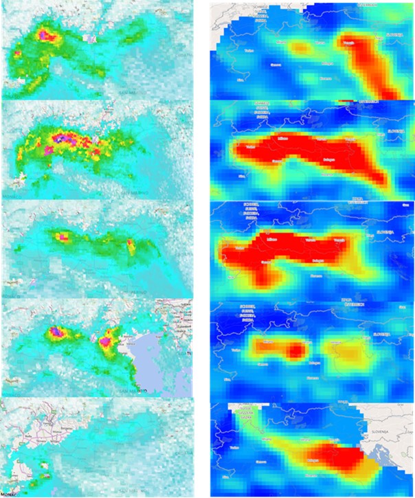
Figure 4.1: TROPOMI (left) and GOME-2 (MetOp-B and -C combined; right) images of tropospheric nitrogen dioxide,
before (12 February), during (15, 16, 21) and after (22) the pollution episode (ADAM Platform).
The satellite images show that this pollution episode does not involve a short intense emission, but an accumulation of pollutants over several days. Selected GOME-2 and S5P TROPOMI images of total column nitrogen dioxide are presented in Figure 4.1. Note that these satellite total column amounts do not provide much information about the actual surface concentration, they are more for qualitative than quantitative usage. Quantitative information at ground level stations can be found, for example, on EEA websites.
Question 19
Why do GOME-2 and TROPOMI produce only one image per day?
Now you can check additional resources to interpret the satellite images and investigate the causes of this air pollution event. Checking multiple resources also helps to estimate how and when the pollution episode might end.
B. Population density (and associated domestic emissions), number and type of industrial sources
The Po basin contains some of Italy's largest cities; economically the region is very important for Italy. It contains a wide variety of pollution sources, which are mainly related to traffic, domestic heating, industry and energy production (see Figure 4.2), agriculture, and farming activities.
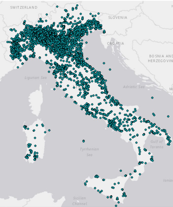
Not surprisingly, the Po basin is one of the European hotspots in terms of suffering from premature mortality associated with atmospheric pollution (EEA, 2015). This region is one of the most densely populated, industrialised, and, therefore, polluted areas in Europe. Pollutant sources include those from urban areas (e.g., Milan), intensive breeding and agriculture, and large manufacturing areas. Hence, for many air pollutants, frequent exceedances of the European limits and target values seem inevitable.
C. Orographic situation
Wind is one of the main driving factors of turbulence and, consequently, dilution of pollutants. Wind speed and direction are influenced by the orography of an area. Figure 4.3 shows an elevation map of the Po valley.
Question 20
When looking at the orographic situation (Figure 4.3), in which part of the basin would you expect the highest accumulation of air pollution? North, South, East, West or in the centre? (Click on the image)
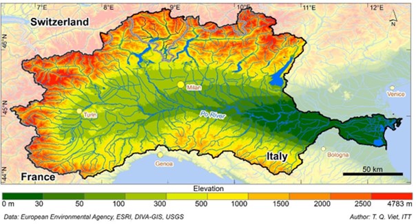
Near central Europe where, in winter, high pressure systems can persist for extended periods, the Po valley is a favourable region for atmospheric stagnation events. The valley morphology exacerbates the effect on air quality, as heavy emissions from industrial activities, as well as from vehicular traffic and residential heating, are often trapped within the Po basin, due to the Alpine chain and the Apennines enclosing the plain on its northern, western, and southern sides. These significant surrounding mountain ranges hinder large-scale horizontal dispersion and long-range transport of pollutants. Additionally, air pollution from the valleys on the southern side of the Alps is transported into the Po basin.
D. Atmospheric conditions
In this case in February 2019, large-scale horizontal atmospheric transport had been limited for about 10 days, as seen in Figure 4.4 below.
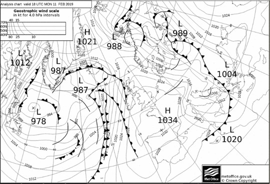
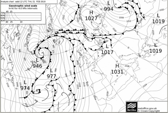
Figure 4.4: Surface synoptic charts for 11 and 21 February 2019 (Wetter3.de) showing a high-pressure area over the Po Valley.
Question 21
Which atmospheric conditions favouring an air pollution event are present?
Question 22
From 21 February onwards, how long do you estimate that the pollution episode will last:
Not uncommonly in February over central south Europe, the synoptic maps show a stagnant high-pressure system. Under such conditions, primary pollutants tend to accumulate and secondary pollutants form in the shallow layer near the surface. For approximately ten days there is a stable atmospheric situation, with a dominant high-pressure system located over northern Italy. Based on the synoptic situation (Figure 4.4), a temperature inversion may have occurred. Such an inversion limits vertical dispersion and, therefore, ventilation into the free troposphere.
During stagnant high-pressure winter conditions, inversions can occur that limit even further the dispersion of air pollutants. To estimate whether an inversion did indeed form, we can look at the soundings. In the Po valley, there are soundings available from three locations in northern Italy: International Airport Cuneo-Levaldigi, Rivolte, and San Pietro Capofiume (Figure 4.5).
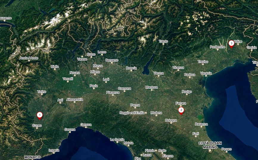
Figure 4.5: Three sounding locations in northern Italy: International Airport Cuneo-Levaldigi (1), San Pietro Capofiume (2), and Rivolte (3) (Mapy.cz).
You can examine the sounding profiles from 21 February from Cuneo-Levaldigi, shown in Figure 4.6. Only daytime temperature inversions are important because they are related to conditions of atmospheric stability; at night, temperature inversions are typically due to the difference in solar radiation between day and night.
Figure 4.6: Skew-T diagrams of sounding profiles at Cuneo-Levaldigi, with the temperature (right black line) and dew-point temperature (left black line), and wind barbs to the right. Clouds are present if the temperature and dew-point temperature just above the boundary layer are equal. (University of Wyoming).
Question 23
Which characteristics of an inversion are visible?
Winds mix the boundary layer and weaken the inversion. The Po Valley basin is characterized by some of the lowest wind speeds in Europe, on average between 2 and 2.5 m s-1, and in winter even lower, around 1.5 m s-1 on average. Temperature inversions are very frequent, especially during cold periods when the height of Planetary Boundary Layer rarely exceeds 450 m.
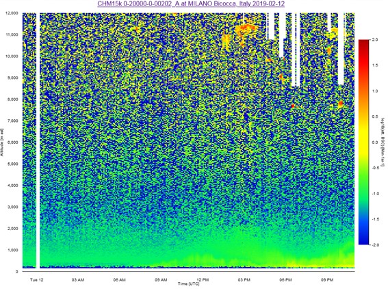
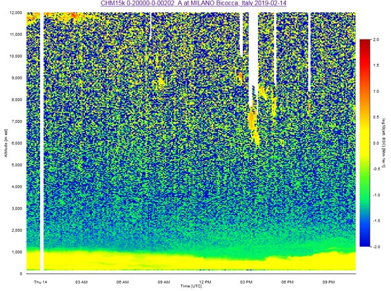
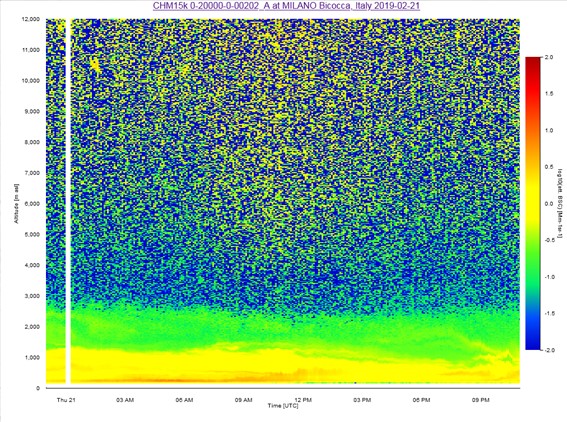
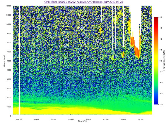
The sounding at Cuneo-Levaldigi, displayed in Figure 4.6, does indeed show the presence of a temperature inversion, but only at night. In this Po Valley case, an inversion is not the only factor causing accumulation of pollutants; nevertheless, the ceilometer plots (Figure 4.7) show an accumulation of aerosols, especially on the 21st compared to the 12th and 14th. On the 25th the aerosol load is reduced again.
Question 24
How do you expect this pollution episode to end?
According to the ceilometer profile, no rain was expected. The AROME model precipitation forecast from 21 February at 15 UTC for the next 12 hours shows very little rain (Figure 4.8). The synoptic charts show a cold front possibly passing from the northeast shortly after 23 February at 06 UTC.
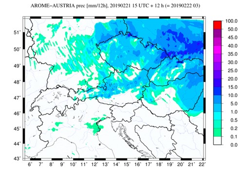
Figure 4.8: AROME Austria, precipitation forecast from 21 February at 15 UTC for the next 12 hours. (GeoSphere Austria)
You could check whether a front did indeed pass by: go to www.wetter3.de and determine whether the pollution episode could have ended due to a front passing. The charts also show that, from 22 February onwards, an easterly flow started to develop.
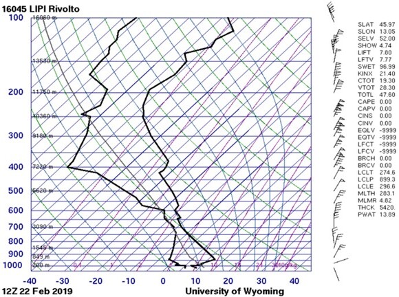
The next information resource that we can check is the sounding, for example at Rivolte, see Figure 4.9. As in the synoptic charts, this plot shows that a strong wind from the northeast started to occur around 22 February at 12 UTC. The soundings in Milan show a clear change in wind speed and direction from 22 February to 23 February: between 200 and 400 m, the wind speed increases from 4-5 knots (2.06-2.57 m s-1) to 10-18 knots (5.14-9.26 m s-1), and the direction changes from 249 (WSW) to 94 (E). It is most likely that this strong wind, occurring for a few days, has ended the pollution episode.
From 26 February, the smog alert was withdrawn and emergency measures were withdrawn in all municipalities belonging to the PAIR of the Emilia-Romagna region. Only Piacenza did not yet meet the conditions for withdrawing the alert (two consecutive days of falling within the legal limits of 50 µg m-3 for the maximum daily concentration of PM10), and therefore the emergency measures remained there until 28 February.
If you would like to learn more about air quality and satellite observations, an EUMETSAT course is available here: www.atmospheremooc.org.