Table of Contents
Cloud Structure In Satellite Images
Secondary Lows appear as a cloud vortex within the frontal cloud band. In this study 23 cases of Secondary Lows within an occluded front were investigated.
The formation of a Secondary Low can be seen in a series of satellite images:
- Initially the cloud thickens, and the whole front seems to be undulating.
- In the development stage, a cloud vortex appears, rotating cyclonically around the Secondary Low.
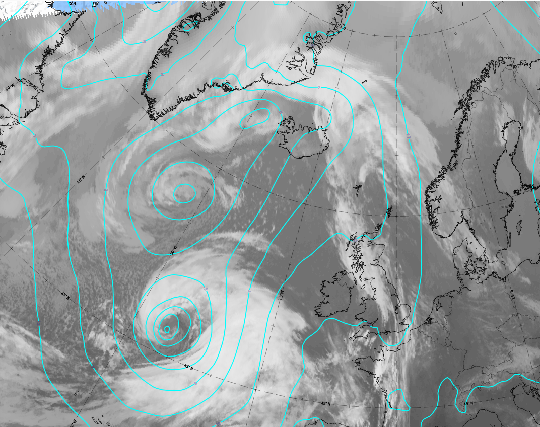
- In the mature stage there are two separate cloud spirals curling around the lows.
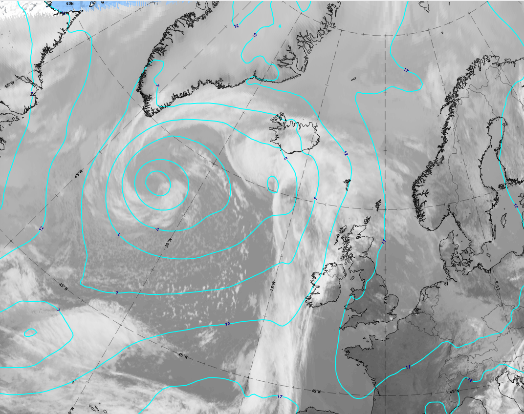
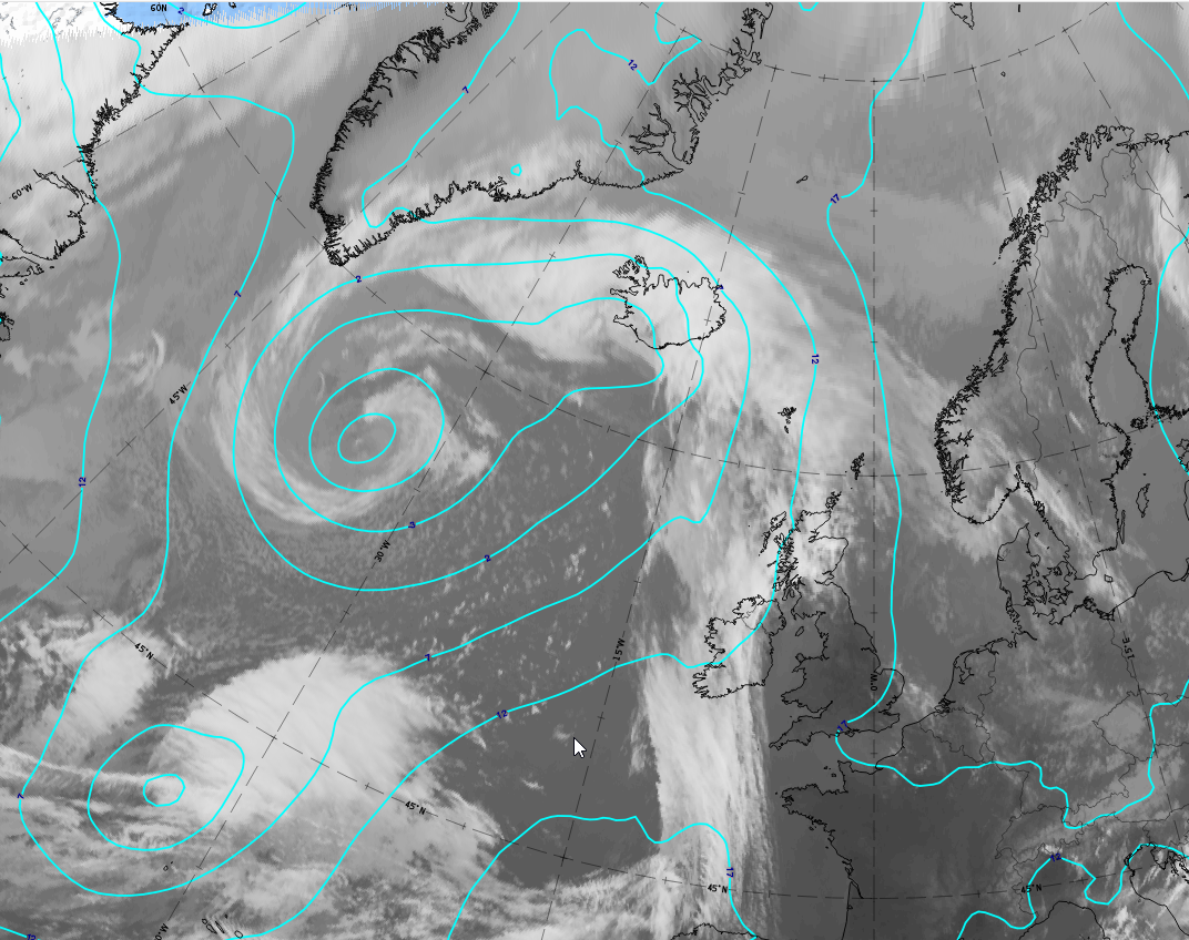
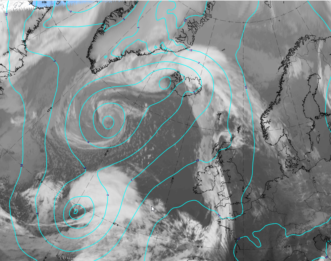
The case of 20 May 2020 includes at 12 UTC a cloud spiral belonging to a large surface low south of Greenland, as well as an area of thicker cloud south-west of Iceland that is connected to a weak surface low. During the next 6 hours a weak spiral structure develops there, which intensifies during the next 12 hours until 6 UTC on 21 May 2020. The mature stage, with two spirals, can be seen from 00 UTC on 21 May 2020 onwards.
 |
 |
 |
 |
Legend:
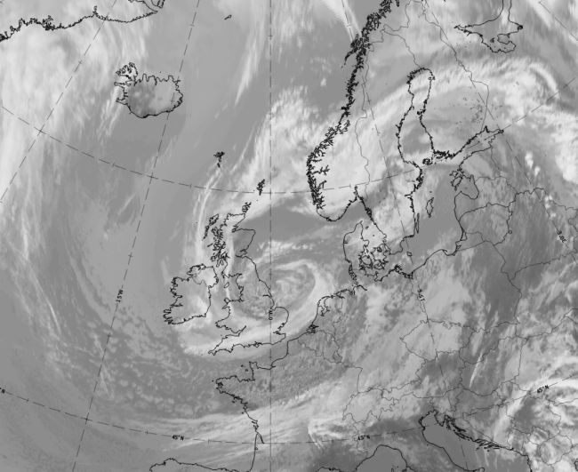
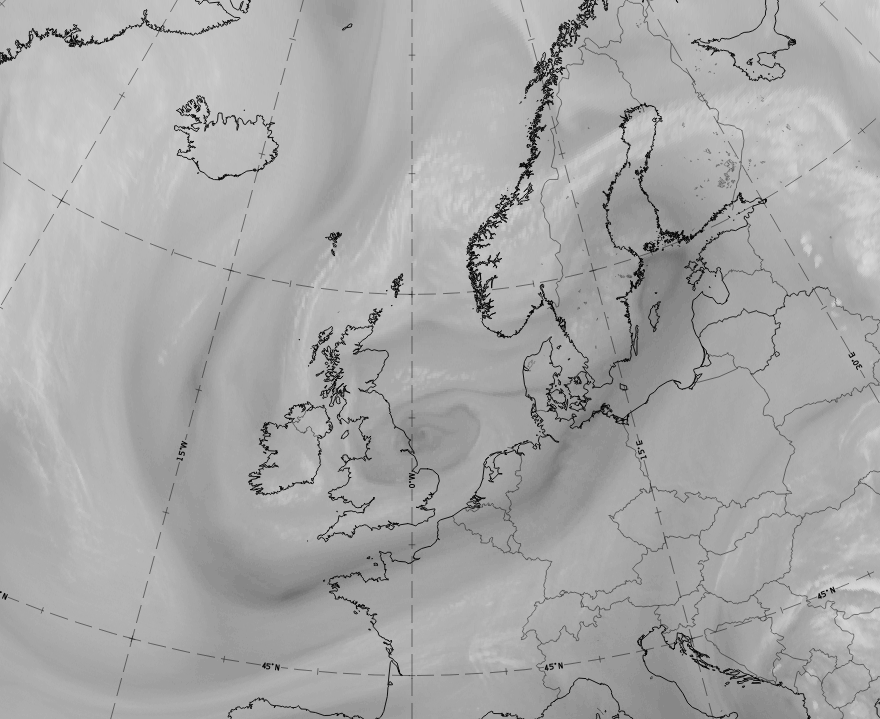
20 - 21 May 2020: 6 hourly sequence of IR images from 12 UTC on 20 May to 06 UTC on 21 May. Contour lines at 1000 hPa are superimposed in cyan.
*Note: click on the image to access the image gallery (navigate using arrows on keyboard).
Appearance in the basic channels:
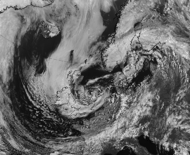
- Visible images are rarely useful, because Secondary Lows within occluded fronts develop mostly over the Northern Atlantic during the winter season, and the daylight time is short. However, if available, the visible or HRV images appear very white in the vicinity of the strengthening second low. During later stages, the old low which is decaying, becomes greyer in the VIS image.
- In infrared images a white to light grey multi-layered cloud spiral develops
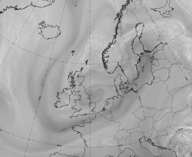
- In water vapour images a white to light grey cloud spiral develops around the Secondary Low. Additionally, there is usually a Dark Eye over it, and a Dark Stripe behind the Cold Front and ahead of the Occluded Front.
Appearance in the basic RGBs:
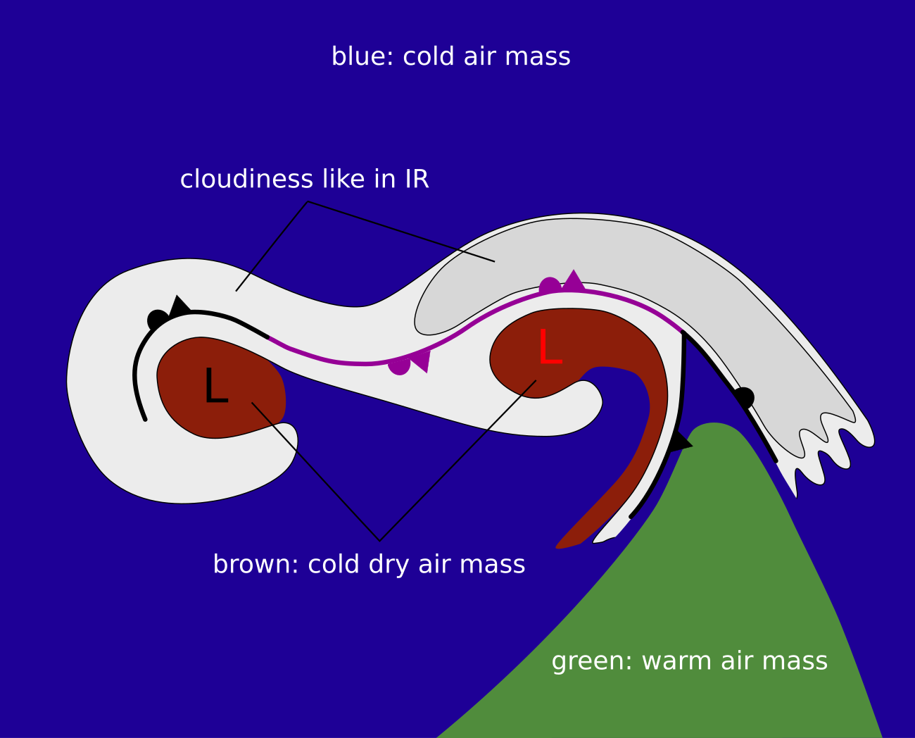
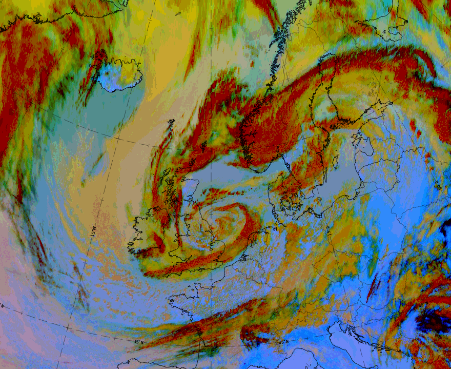
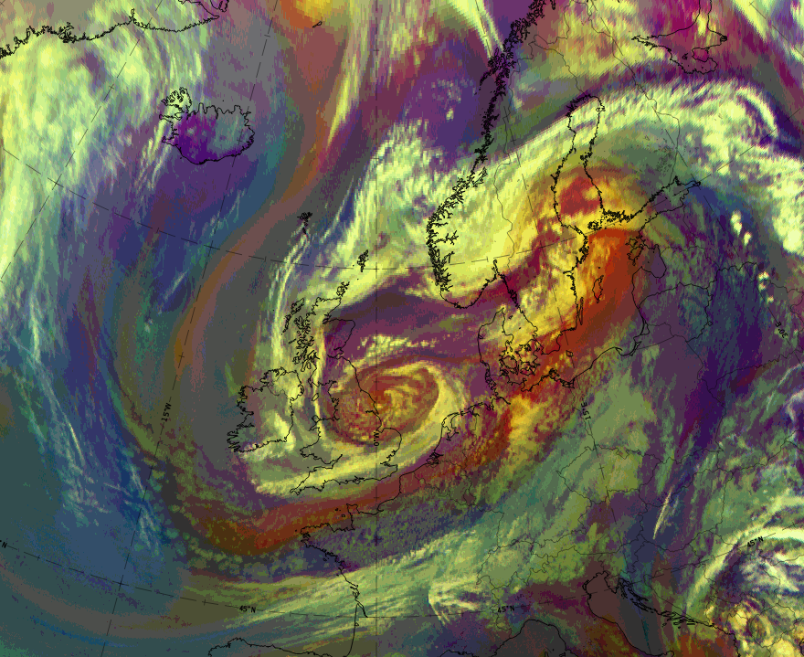
Airmass RGB
The mostly elongated occlusion cloud band, as well as the two embedded cloud spirals, are within an area of blue and dark brown colours, indicating cold and dry airmasses. The cold airmasses in blue are more to the north and north-west of the occlusion cloud system, while the centres of the spirals appear in the dark brown colours of cold and dry air. In most cases the second occlusion spiral centre has more intensive bright colours while the dark brown colour in the primary spiral centre, which is older and filling up, is less intensive. Greenish colours indicate warmer air masses more to the south of the cloud systems.
The cloud bands and spirals look similar to those in the IR image.
Dust RGB
Cloud systems of an occlusion cloud band and embedded spirals are surrounded by blue colours, where the air is cloud-free. In more northern latitudes there are many ochre-coloured areas, indicating low- to mid-level cloud.
The clouds of this system appear in ochre to dark red colours. Usually, the cloud belonging to the second low is dark red indicating thick ice cloud, there while the primary older cloud spiral looks more ochre with dark red cloud fibres above. It consists mostly of mid-level clouds with remnants of thick ice cloud above.
 |
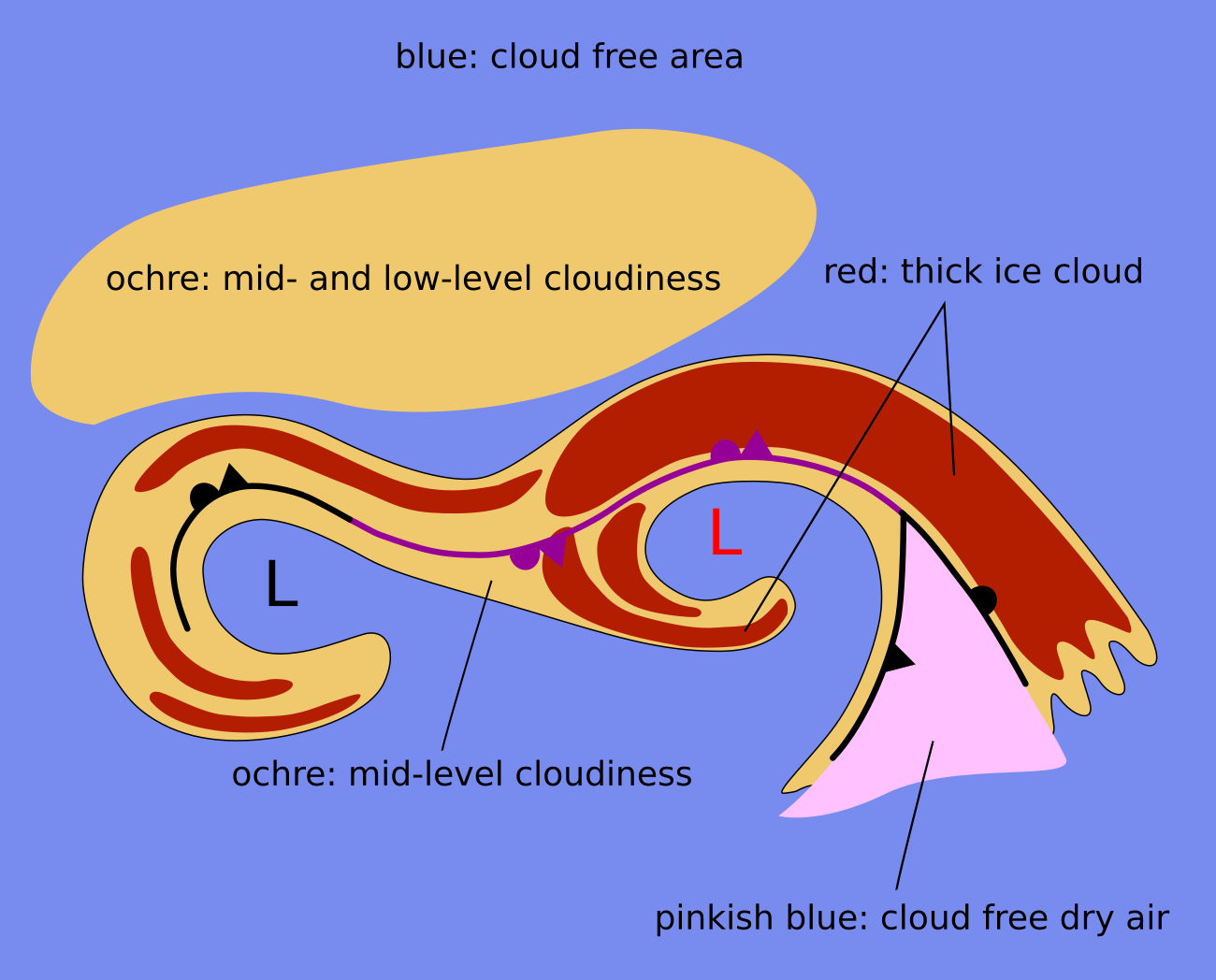 |
Legend: basic RGB Schematics.
Left: Airmass RGB; right: Dust RGB.
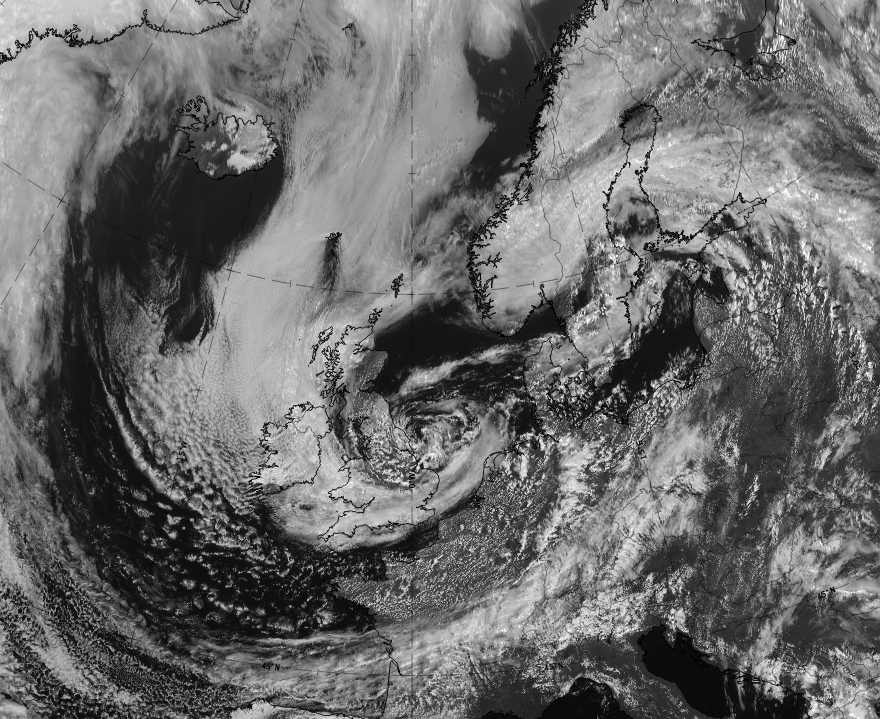
In the case of 6 June 2020 at 12 UTC, the cloud band of an occlusion extends from central Finland across mid-Scandinavia where the spiral of the second low has formed, and further west- and south-westward to the British Isles and into the North Sea where the centre of the primary low spiral is centred.
|
|
|
|

6 June 2020, 12 UTC: 1st row: IR (above) + HRV (below); 2nd row: WV (above) + Airmass RGB (below); 3rd row: Dust RGB + image gallery.
*Note: click on the image to access the image gallery (navigate using arrows on keyboard)
| IR | Bright white within the whole cloud band and the spirals. More fibrous texture in the primary cloud spiral. |
| HRV | Bright white, especially in the eastern part and the secondary cloud spiral. Grey areas in between the two spirals. |
| WV | Dark grey areas in the centres of the two cloud spirals, indicating the sinking dry air. |
| Airmass RGB | Dark brown areas in the centres of the two cloud spirals. More distinct colours in the centre of the Secondary Low; a mixture of dark blue and dark brown colours within the centre of the primary low. This illustrates the life cycle of the two lows, with a developing and a decaying stage |
| Dust RGB | Dark red colours within both cloud spirals. More extended bright areas in the cloud of the Secondary Low, but more fibres in the primary low. Ochre colours indicate the mid-level cloud. |
Meteorological Physical Background
The formation of a Secondary Low within an Occluded Front has three prerequisites:
- A distinct maximum of vorticity both shear and curvature components are usually present)
- There is a jet streak on the cyclonic side of the occluded front and parallel to it
- Wind velocities in the jet streak are at least 50 m/s
A Secondary Low often forms (in 65% of the cases) within a Neutral Occlusion, that is, the Occlusion is neither warm nor cold (compare Occlusion: Cold Conveyor Belt Type - Meteorological physical background ). In this type a strong jet runs over the Occlusion point. The low forms usually between the Occlusion point and the midpoint of the occluded Front.
Nearly all Secondary Lows form in systems over the sea during the winter season. This follows from the fact that the basic westerly flow is stronger during the winter, and the deepening of a low is easier over the relatively warm water.
Although the secondary lows are associated with strong jets, the processes in the left exit region are involved in less than half of the cases. But if the left exit region is favourably situated in the vicinity of the occluded front, it can enhance the development, as in the case on 07 February 2002.
In the process of the secondary low development there is temporarily a back bent part in the occluded Front. The situation, however, is different from the conceptual model Back - Bent Occlusion (see Back - Bent Occlusion - Meteorological physical background ).
Three stages can be distinguished in the development of a Secondary Low within an occluded front:
- Initial stage A Secondary Low begins to deepen within the occluded front in the area of a local vorticity maximum. The part of the front around the low has a Wave - like structure for a short time (compare Wave ). This Wave does not amplify, however, but turns into an Occlusion spiral.
- Developing stage Whilst the original low fills up, the secondary deepens. At this stage the occluded front with the Secondary Low still moves forward.
- Mature stage The occluded front splits into two parts that spiral around their respective lows. The movement of the Secondary Low slows and it begins to fill up.
The case of 17 of April 2008:
Below, initial stage at 00.00 UTC: There is an area of a local vorticity maximum and thick frontal cloudiness west of France, where the Secondary Low begins to deepen.
|
17 April 2008/06.00 UTC - Meteosat 9 IR image; magenta: height contours 1000 hPa, cyan: relative vorticity 500 hPa
|
|
|
|
Below, developing stage at 12.00 UTC: A deep low pressure centre lies over the Bay of Biscay.
|
17 April 2008/12.00 UTC - Meteosat 9 IR image; magenta: height contours 1000 hPa, cyan: relative vorticity 500 hPa
|
|
|
|
Below, mature stage on 17 April 2008 at 18.00 UTC: The Secondary Low is over Brittany.
|
17 April 2008/18.00 UTC - Meteosat 9 IR image; magenta: height contours 1000 hPa, cyan: relative vorticity 500 hPa
|
|
|
|
Key Parameters
- Height contours at 1000 hPa:
On the surface there is an elongated low pressure area connected to a long occluded front. The original low centre is separated from the occluded front, whereas the secondary centre develops within the frontal cloud band. - Equivalent thickness at 500-850 hPa:
There is the typical structure of an Occlusion, and usually the thermal structure of the Occlusion is neutral, see e.g. Occlusion: Warm Conveyor Belt Type (compare Occlusion: Warm Conveyor Belt Type ). In all types of Occlusions there is a thickness ridge along the occluded front. - Omega at 700 hPa:
There is ascending motion related to the whole frontal system, but also a distinct maximum over the deepening Secondary Low. - 300 hPa Isotaches at 300 hPa:
The core of the jet stream crosses the occlusion point, and the strength of the jet streak is at least 50 m/s.
In the images below the Secondary Low is marked by a red arrow.
Height contours at 1000 hPa and equivalent thickness at 500 - 850 hPa
|
17 April 2008/12.00 UTC - Meteosat 9 IR image; magenta: height contours 1000 hPa, green: relative topography 500 - 850 hPa
|
|
|
|
Omega at 700 hPa
|
17 April 2008/12.00 UTC - Meteosat 9 IR image; yellow: omega
|
|
|
|
Isotachs at 300 hPa
|
17 April 2008/12.00 UTC - Meteosat 9 IR image; yellow: isotachs 300hPa
|
|
|
|
Typical Appearance In Vertical Cross Sections
- Isentropes:
The structure of an Occlusion is seen in the isentropes. As the Occlusions can be fairly old, however, the v-shaped structure with warmer isentropes above may not always be as clear as in younger systems. - Divergence:
As in a typical deepening low, there is convergence at low levels and divergence at high levels over the secondary low. - Positive vorticity advection:
There is a maximum on PVA ahead of the developing low in the lower troposphere.
|
17 April 2008/10.00 UTC - Meteosat 9 IR image; position of vertical cross section indicated
|
|
|
|
|
17 April 2008/12.00 UTC - Vertical cross section; black: isentropes (ThetaE), magenta thick: convergence, magenta thin: divergence
|
|
|
|
|
17 April 2008/12.00 UTC - Vertical cross section; black: isentropes (ThetaE), green: positive vorticity advection (PVA)
|
|
|
|
Weather Events
The Secondary Low Centre within an occluded front is accompanied by rain, showers and possibly thunder.
| Parameter | Description |
| Precipitation |
|
| Temperature |
|
| Wind (incl. gusts) |
|
| Other relevant information |
A case on 6 June 2019 at 12 UTC demonstrates the weather features.
|
|
Legend:
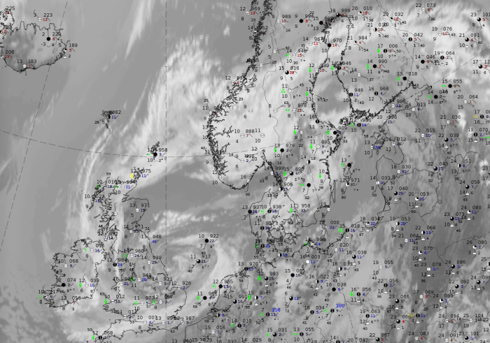
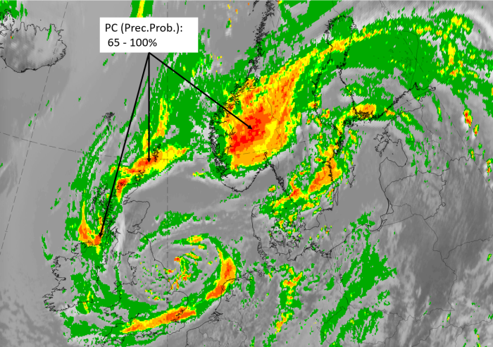
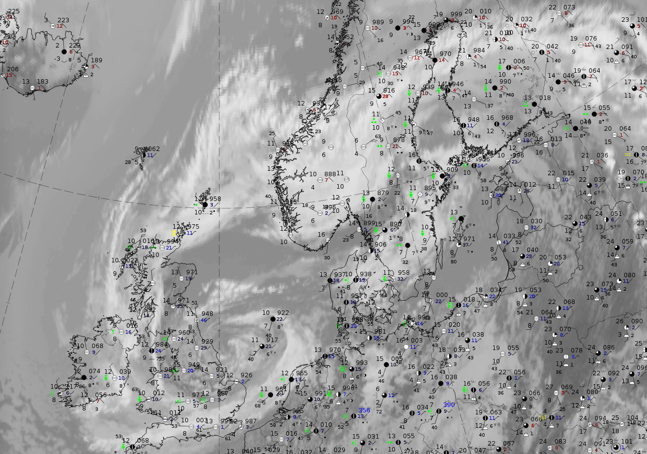
27 September 2019, 12UTC: IR + synoptic measurements (above) + probability of moderate rain (Precipitting clouds PC - NWCSAF).
Note: for a larger SYNOP image click this link.
Synoptic observations of rain and showers occur in the whole band and spiral system but the intensity is clearly higher in the cloud of the Secondary Low system than in that of the older primary low. The precipitation probabilities computed by the NWCSAF are very high in both regions (up to 100%). However, this parameter shows wide areas of these high probabilities in the secondary cloud spiral, with only a few spots in the primary cloud spiral.
|
|

|
|
Legend:
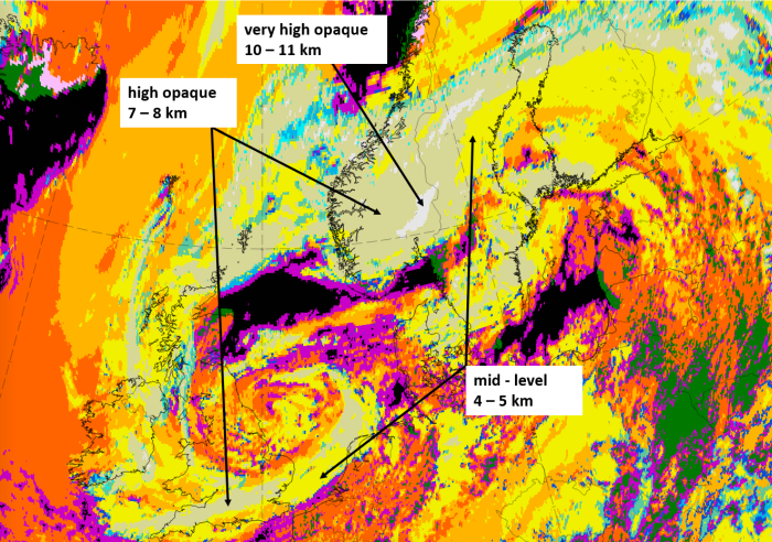
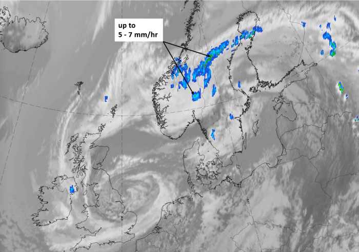
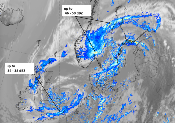
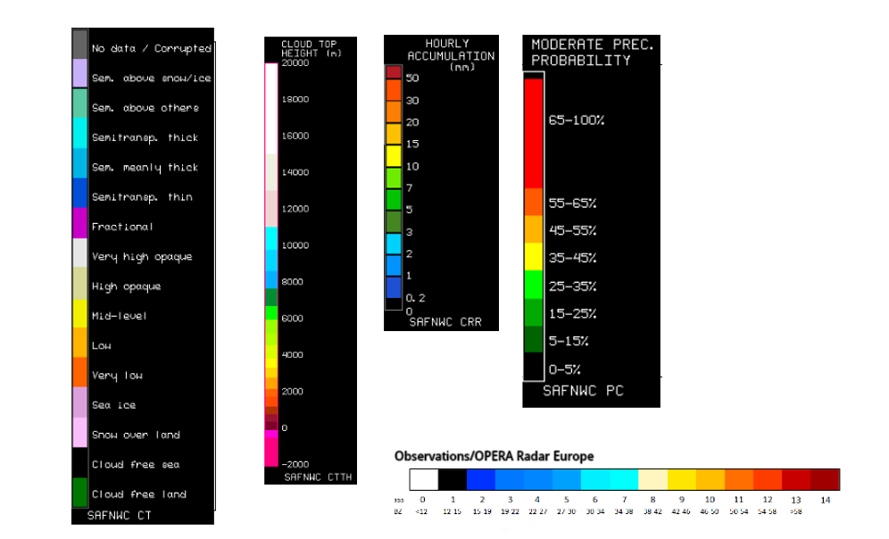
6 June 2020, 12 UTC; IR, with the following fields superimposed:
1st row: Cloud Type (CT NWCSAF) (above) + Cloud Top Height (CTTH - NWCSAF) (below); 2nd row: Convective Rainfall Rate (CRR NWCSAF) (above) + Radar intensities from Opera radar system (below).
For identifying values for Cloud type (CT), Cloud type height (CTTH), precipitating clouds (PC), and Opera radar for any pixel in the images look into the legends. (link)
References
General Meteorology and Basics
- CARR W. M. (1999): International Marine's Weather Predicting Simplified: How to Read Weather Charts and Satellite Images; McGraw-Hill
General Satellite Meteorology
- BADER M. J., FORBES G. S., GRANT J. R., LILLEY R. B. E. and WATERS A. J. (1995): Images in weather forecasting - A practical guide for interpreting satellite and radar imagery; Cambridge University Press.