Table of Contents
Cloud Structure In Satellite Images
Shapiro-Keyser cyclones are most frequently observed over the oceans. The life cycle of a Shapiro-Keyser cyclone substantially differs from the that of a Norwegian-type cyclone. This difference is less obvious when looking at satellite imagery, but it becomes more apparent when looking at the NWP parameters that naturally reflect the ongoing physical processes. These differences are most pronounced during the intensification and the mature stages.
Shapiro-Keyser cyclones often show a rapid development and a strong deepening of the surface low, for which reason they often fulfil the criterion of Rapid Cyclogenesis. When the deepening of the surface low within 24 hours exceeds a given threshold, they are classified as Rapid Cyclogenesis. This threshold depends on the geographical position of the system; the classification criterion is as follows:
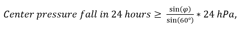
where φ is the geographical latitude of the system.
As for the Norwegian cyclone, we define five development stages in the life-cycle of a Shapiro-Keyser cyclone:
- Initial stage
- Wave stage
- Intensification stage
- Mature stage
- Dissipation stage
However, in this manual the starting point is the satellite images, and as the air mass boundary in the initial stage (1) is often cloud-free or accompanied by randomly arranged cloud patches without any typical structure, it will not be treated in this and the following chapters. Schematics and cases representing the process of cyclogenesis will therefore start with the wave stage (2), where cloud systems already show a more organized structure and can be properly identified in satellite imagery.
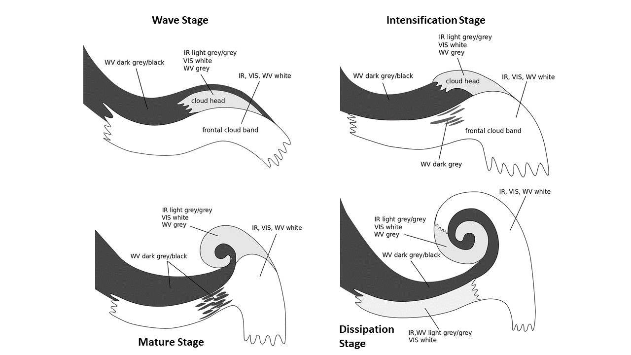
Figure 1: Schematics of the development stages of a Shapiro-Keyser cyclone as depicted in the SEVIRI channels IR 10.8 μm, WV 6.2 μm and HR-VIS.
Appearance in SEVIRI channels IR 10.8 μm, WV 6.2 μm and HR-VIS:
Wave stage:
When the frontal zone starts to form a wave, the frontal cloud band is organized into regions with cyclonic and anticyclonic curvature, which correspond physically to a cold and a warm front, respectively. In this very early stage of the cyclone development, a cloud head emerges at the rear of the transition zone from cold to warm front. This cloud head can be clearly distinguished in IR imagery from the main cloud band because of its lower cloud tops.

Figure 2: Schematics of the wave stage of a Shapiro-Keyser cyclone as depicted in the SEVIRI channels IR 10.8 μm, WV 6.2 μm and HR-VIS.
IR 10.8 μm channel:
- Two main cloud configurations are seen during the wave stage of cyclogenesis: (1) a frontal cloud band usually oriented east to west, and (2) a so-called "cloud head", on the poleward side of the frontal cloud band, protruding from beneath it. The shades of the developing cloud head varies between grey and light grey in the IR channels, mostly with higher tops on the poleward side.
- Dry air originating from higher atmospheric levels descends on the cyclonic side of a jet stream at the rear of the frontal cloud band. This leads to a dark, cloud-free area between the cloud band of the cold front and the cloud head, thereby creating a V-pattern (often also called a dry slot).
WV 6.2 μm channel:
- A dark stripe usually accompanies the formation of a Shapiro-Keyser cyclone. In WV imagery, this dark stripe is located at the rear of the "cold frontal" cloud band in the wave stage.
- The dark stripe occurs at the cyclonic side of the jet stream. Before the development starts, the dark stripe is more distinct upstream of the cloud head.
VIS channel:
- Visible imagery is not well suited to a frontal analysis. Nevertheless, the development of the Shapiro-Keyser system can be monitored from the early wave stage until the final dissipation stage using VIS imagery. The frontal cloud band and the cloud head appear in light grey shades, while the cloud-free areas, especially the dry slot that forms when the cloud head separates from the frontal cloud band, appear darker grey.
Intensification stage:
During the intensification stage of the Shapiro-Keyser cyclone, the curvature of the frontal cloud band accentuates. The cloud head grows larger and starts to separate from the front, with a cloud-free gap opening between the cold front and the rear part of the cloud head. The height difference between the frontal cloud band and cloud head persists.

Figure 3: Schematic of the intensification stage of a Shapiro-Keyser cyclone as depicted in the SEVIRI channels IR 10.8 μm, WV 6.2 μm and HR-VIS.
IR 10.8 μm channel:
- The frontal cloud band consists of high-reaching clouds and appears in white scales in the IR imagery while the cloud head appears in grey scales typical for mid-level cloud heights.
WV 6.2 μm channel:
- When the cloud head detaches from the frontal cloud band during the intensification stage, the dark stripe fills the gap (V-pattern).
VIS channel:
- As the frontal cloud band consists of higher clouds than those of the cloud head, the frontal clouds can cast a distinct shadow on the cloud head, this is visible in VIS imagery.
Mature stage:
During the mature stage of the Shapiro-Keyser cyclone the cloud head transforms into an occlusion-like cloud band that wraps around the low-pressure core of the Shapiro-Keyser cyclone. At the same time, it intensifies and reaches higher atmospheric levels.
The angle between the cold and warm front narrows and reaches about 90° so that they become perpendicular. This pattern, characteristic for this cyclone type, is called a T-bone pattern.
In the mature stage, the warm front is far more clearly visible than the cold front. The cold front often has a patchy structure, and sometimes only consists of high clouds (e.g., an upper-level cold front) with reduced vertical extent.
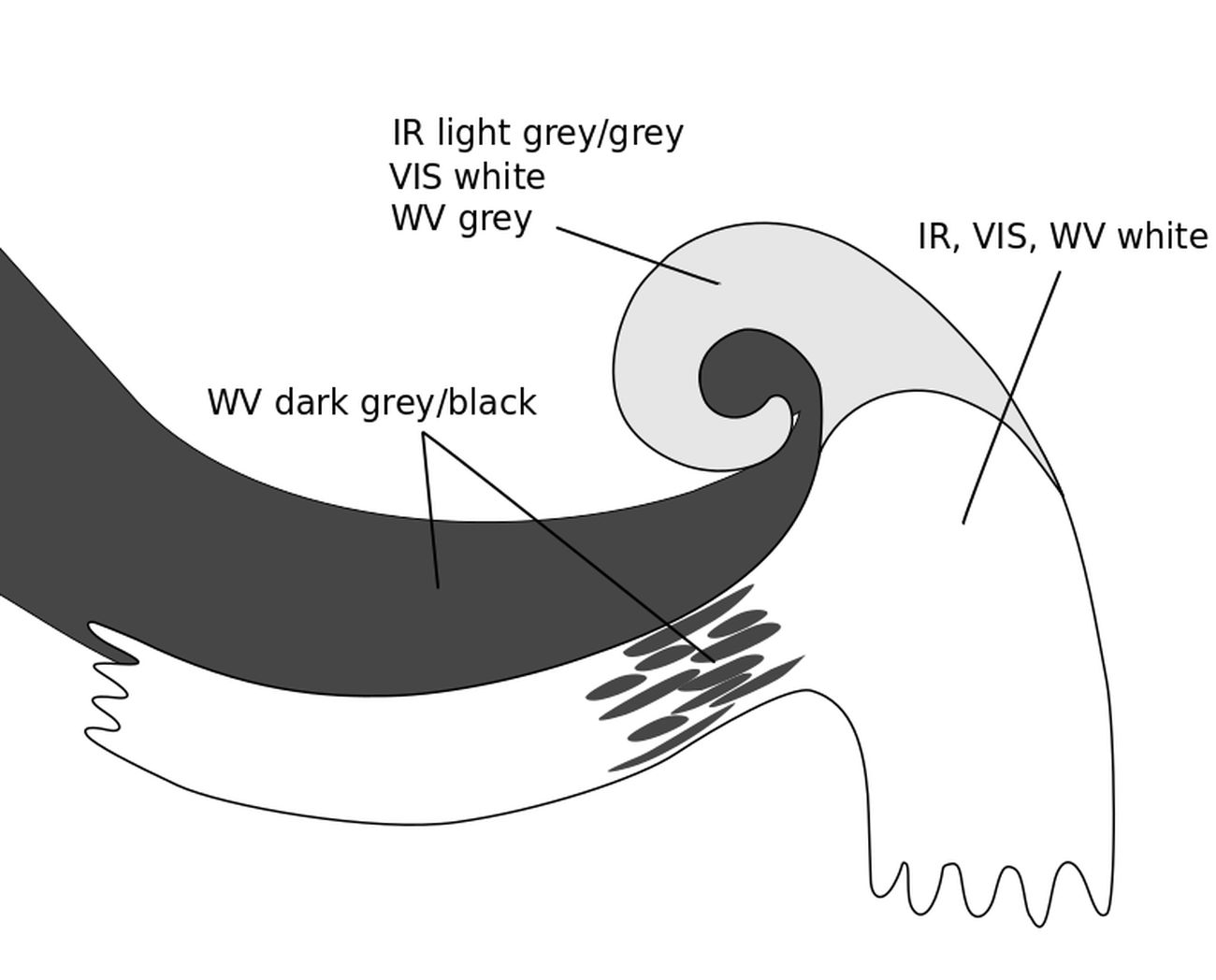
Figure 4: Schematics of the mature stage of a Shapiro-Keyser cyclone as depicted in the SEVIRI channels IR 10.8 μm, WV 6.2 μm and HR-VIS.
IR 10.8 μm channel:
- With the deepening of the surface low in the mature phase, the cloud head detaches from the frontal cloud band and becomes more spiral like in structure. At the same time as the cloud band wraps around the system core, its appearance becomes whiter in the IR imagery.
WV 6.2 μm channel:
- During the mature stage, the cloud head grows into a cyclonically curved cloud spiral with a broad dark area between the spiral and the frontal cloud band. Compared to the intensification stage, the dark stripe becomes greyer and the contrast reduces.
- Another dark stripe that is connected to a second jet streak can be observed ahead of the warm front.
VIS channel:
- The frontal cloud bands are depicted in bright grey shades and the cold front has a less compact structure than the warm front.
Dissipation stage:
During the dissipation stage, the Shapiro-Keyser cyclone strongly resembles the Norwegian cyclone type from the satellite perspective. The former cloud head, now very similar to a classical occlusion cloud band, wraps around the system core and dissipates slowly.

Figure 5: Schematic of the dissipation stage of a Shapiro-Keyser cyclone as depicted in the SEVIRI channels IR 10.8 μm, WV 6.2 μm and HR-VIS.
IR 10.8 μm channel:
- While the warm front is more persistent in IR imagery, the cold front and the occlusion-like cloud band dissolve first. Parts of the cloud spiral disappear as the temperature contrast between the warm core and the surrounding air reduces to zero.
WV 6.2 μm channel:
- The contrast between the dark stripe and the surrounding air reduces.
VIS channel:
- The dissipation process is also visible in VIS imagery as the cloud structure becomes patchier and less compact.
Appearance in Airmass RGB:
The composite image that best represents the Shapiro-Keyser cyclogenesis prcess is the Airmass RGB.
- Reddish brown colours are found in the cold air behind the cold front. They represent dry, sinking air masses, which typically occur in a dry intrusion. They are often co-located with the jet stream.
- Frontal cloud bands are depicted in white unless they are overrun by the dry intrusion. In that case, they have a reddish white colour.
- Cold air masses are typically represented in blue tones, while warmer, tropical air masses are depicted in green.
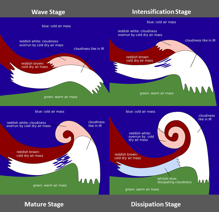
Figure 6: Schematics of the development stages of a Shapiro-Keyser cyclone as depicted in the Airmass RGB.
During the period of 2 to 4 March 2022, a Shapiro-Keyser cyclone developed over the Atlantic Ocean.
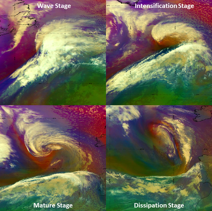
Figure 7: 2 - 4 March 2022, Airmass RGB.
Wave stage: 2 March 2022 at 21:00 UTC - intensification stage: 3 March 2022 at 18:00 UTC;
mature stage: 4 March 2022 at 09:00 UTC; dissipation stage: 4 March 2022 at 21:00 UTC.
The IR 10.8 μm band shows the development of an occlusion-like cloud band (in fact a warm front) around the warm core of the Shapiro-Keyser-system. Cloud fibres can be seen at the rear side of the cold front, indicating the position of the jet.
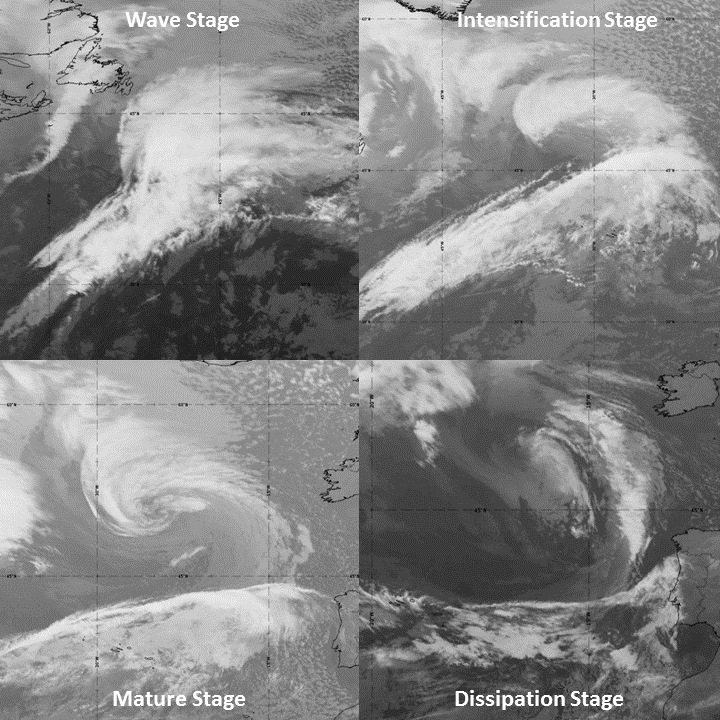
Figure 8: 2 - 4 March 2022, IR 10.8 μm.
Wave stage: 2 March 2022 at 21:00 UTC - intensification stage: 3 March 2022 at 18:00 UTC;
mature stage: 4 March 2022 at 09:00 UTC; dissipation stage: 4 March 2022 at 21:00 UTC.
The water vapour band WV 6.2 μm shows dry sinking air masses (dark areas) behind the cold front and wrapping around the warm core of the Shapiro-Keyser system. During the intensification stage, the dry intrusion is strongest in the cloud-free gap opening between the cold front and the cloud head.
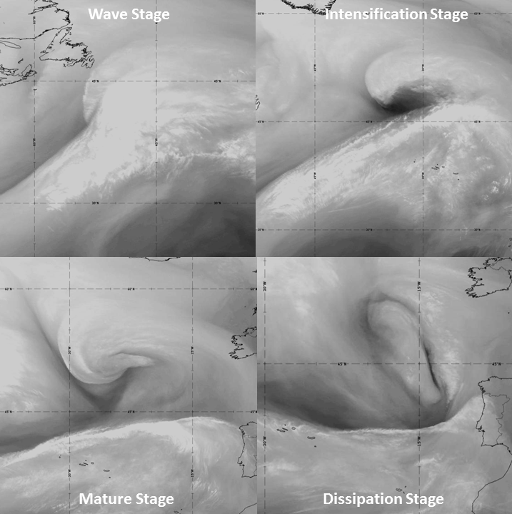
Figure 9: 2 - 4 March 2022, WV 6.2 μm.
Wave stage: 2 March 2022 at 21:00 UTC; intensification stage: 3 March 2022 at 18:00 UTC;
mature stage: 4 March 2022 at 09:00 UTC; dissipation stage: 4 March 2022 at 21:00 UTC.
Bright pixel values show the positions of the fronts in visible imagery. At low solar altitudes, the shadows cast on the cloud tops provide a kind of 3-D effect.
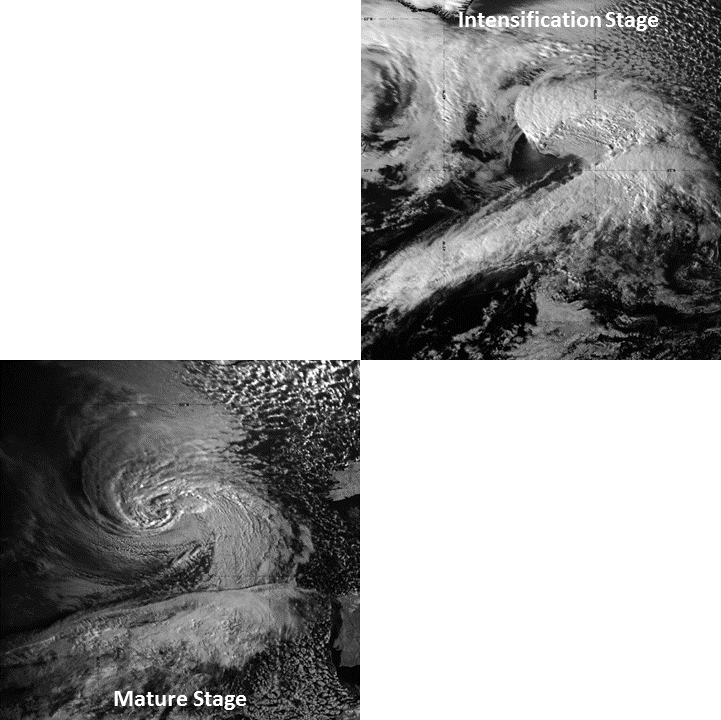
Figure 10:2 - 4 March 2022, VIS 0.8 μm.
Intensification stage: 3 March 2022 at 18:00 UTC; mature stage: 4 March 2022 at 09:00 UTC.
Meteorological Physical Background
In contrast to the Norwegian cyclone type, where the depiction of the cold and the warm front can be reduced to a 2-dimensional sketch, a 3-dimensional perspective is needed to fully understand the physical processes involved in Shapiro-Keyser cyclones. In particular, it is important to differentiate between upper-level and surface fronts. During the evolution of Shapiro-Keyser cyclones, upper-level cold fronts clearly separate from their lower-level counterparts. This forms an essential constituent of the development and evolution of a Shapiro-Keyser cyclone.
For the conveyor belt theory that is applicable to both the Norwegian and the Shapiro-Keyser cyclone models, see here.
Detailed frontal analysis of the Shapiro-Keyser cyclone model
In the Norwegian cyclone model, which is more or less a description of moving air masses, the cold front catches up the warm front during the evolutionary process. The warm air is wrapped around the cold core of the system while simultaneously being lifted.
Shapiro-Keyser cyclones, in contrast, have a warm core and the catch-up process does not take place, at least not until the dissipation phase of the evolution. Hence, occlusions do not play a major role in the evolutionary process: cold and warm fronts suffice to describe this cyclone type.
In order to describe the life cycle of a Shapiro-Keyser cyclone, we adopt the same four evolutionary stages as for the Norwegian cyclone :
- Wave stage
- Intensification stage
- Mature stage
- Dissipation stage

Figure 1: The four stages in the evolution of a Shapiro-Keyser cyclone, from the wave stage to the dissipation stage.
The most important differences between Norwegian and Shapiro-Keyser cyclones occur during stages 2 and 3 (i.e., the intensification and mature stages), while during stage 4, the dissipation stage, the development of the two cyclone types converges again.
Generally, Norwegian cyclones have a pronounced cold front and a less significant warm front, while Shapiro-Keyser cyclones have a strong warm front and a weaker surface cold front.
The intensification stage
During the intensification stage, the main differences between the Norwegian and Shapiro-Keyser cyclone models begin to appear. While for the Norwegian cyclone, the warm sector starts to narrow, leaving the cyclone centre in cold air, we find the Shapiro-Keyser cyclone centre invaded by warm air at lower levels, with a gap (frontal fracture) opening between the cold and the warm front. The warm front starts to wrap around the pressure minimum, delimiting the warm core from the surrounding cold air masses. In reality, the cold and warm front are still connected by an inactive air mass boundary that is usually not drawn on synoptic charts. This air mass boundary often shows a weaker temperature gradient then the cold front (see the grey line in Figure 2 below).
As the warm air protrusion mainly occurs in low to middle atmospheric levels, the upper part of the cold front above the protrusion remains intact and persists as an upper-level cold front (see the light blue cold front in Figure 2 below).
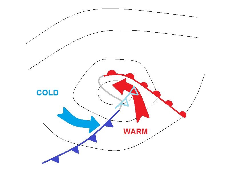

Figure 2:
Left: Schematic of the cold and warm surface front during the intensification phase. The grey line shows the cold frontal fracture.
Right: IR 10.8 μm imagery from 30 November 2021 at 21:00 UTC. Mean surface pressure (black) and ThetaE at 700 hPa (blue and red isolines).
During the early stages of the cyclone development, we usually find two jet streaks: the first is located behind the cold front and the other lies ahead of the warm front. At the beginning of the intensification stage, the jet streaks are nearly parallel to each other. This usually leads to the observation of a jet streak coupling, i.e., the left exit region of one jet streak is located at the right entrance region of the other jet (see Figure 3). Hence, upward motion in this area is reinforced.
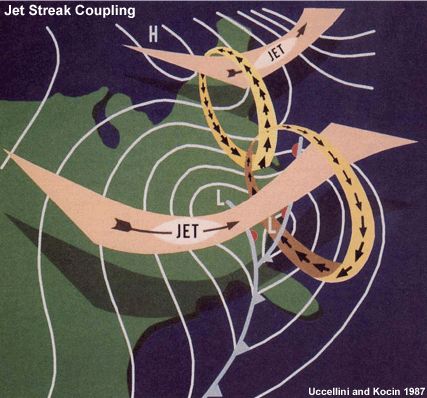
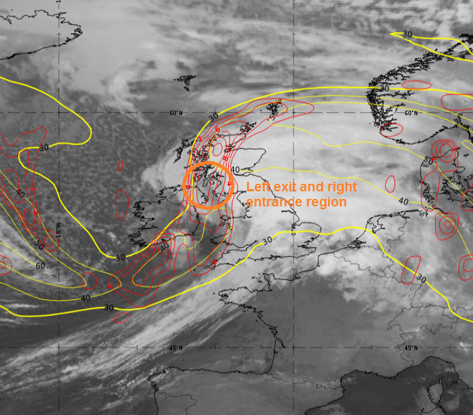
Figure 3:
Left: Schematic of two coupled jet streaks.
Right: IR 10.8 μm imagery from 30 November 2021 at 21:00 UTC. Isotachs and cyclonic vorticity advection at 300 hPa.
The mature stage
During the mature stage, the warm core of the Shapiro-Keyser cyclone becomes secluded from the warm sector by cold air masses advancing from the rear of the cold front (see Figure 4). The warm front around the warm core intensifies and the cold frontal fracture becomes narrower.
The protruding cold air (blue arrows in the schematic below) starts at higher levels and is triggered by the jet streak. Referring to the conveyor belt model, this is the so-called dry intrusion . The dry intrusion affects progressively lower atmospheric levels and hence contributes to the progressing of the cold front in direction of the warm front. The supply of warmer air masses from the warm sector into the system core gradually ceases.
The warm and cold front form a right angle, the so-called T-bone pattern characteristic of Shapiro-Keyser cyclones. There is no occlusion at this stage of development.
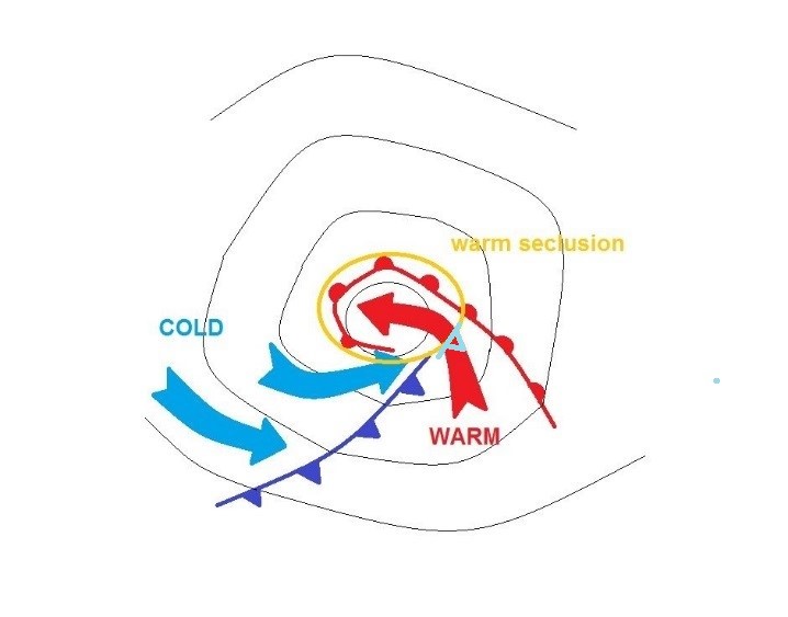
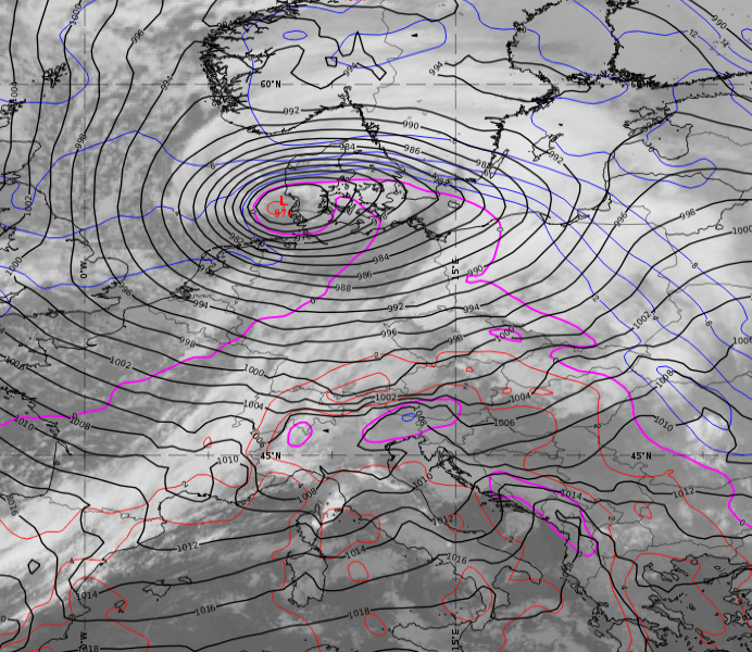
Figure 4:
Left: Positions of the cold and warm fronts during the mature stage. Red and blue arrows mark the advancing air masses.
Right: IR 10.8 μm imagery from 1 December 2021 at 15:00 UTC. Mean surface pressure (black) and temperature at 850 hPa (blue and magenta isolines).
During the mature stage, the angle between the two jet streaks becomes almost 90° (see Figure 5). The coupling of the jet streaks thereby weakens and the deepening of the surface low decelerates.
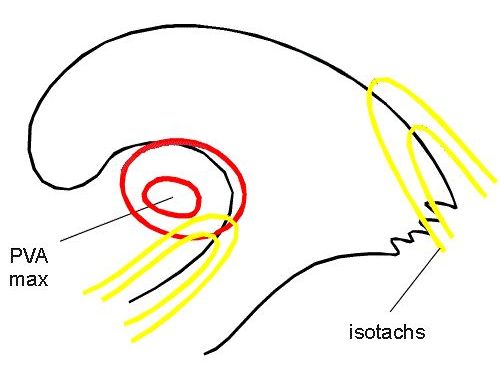
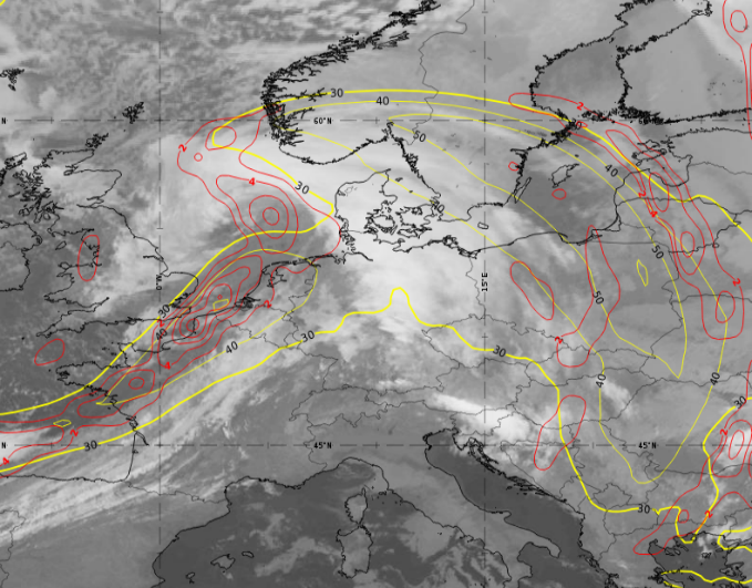
Figure 5:
Left: Schematic of the jet streak positions and the positive vorticity advection maximum (PVA max) at 300 hPa during the mature stage.
Right: IR 10.8 μm imagery from 1 December 2021 at 06:00 UTC. Isotachs at 300 hPa in yellow and PVA at 300 hPa in red.
The dissipation stage
The dissipation phase of the Shapiro-Keyser cyclone is characterized by:
- An increasing surface pressure at the system core;
- A secluded warm core;
- The cold front rejoining the warm front;
- A weakening warm front around the warm core.
During the dissipation stage, cold air protruding from behind the cold front wraps around the warm core of the Shapiro-Keyser cyclone. The warm core of the cyclone is located in the polar air mass and the temperature gradient to this surrounding colder air mass decreases.
Aging Shapiro-Keyser cyclones follow physical processes typical of Norwegian cyclones, such as the merging of the warm and cold fronts to form an occlusion. This is the case when cold air from behind the cold front wraps around the warm core. Subsequently, the cold front connects to the warm front (closing the cold frontal fracture) and forms an occlusion.
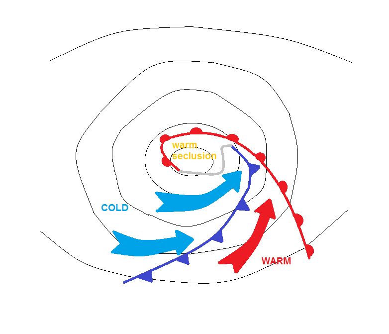
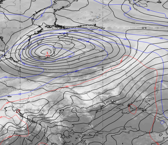
Figure 6:
Left: Schematic of the cold and warm surface front during the dissipation phase. Red and blue arrows mark the advancing air masses.
Right: IR 10.8 μm imagery from 2 December 2021 at 12:00 UTC. Mean surface pressure (black) and ThetaE at 700 hPa (blue and red isolines).
The left-exit quadrant of the jet is no longer superimposed on the surface pressure minimum; upper-level divergence ceases to act as a trigger for the surface low. The two jet streaks are aligned at a more acute angle then before.
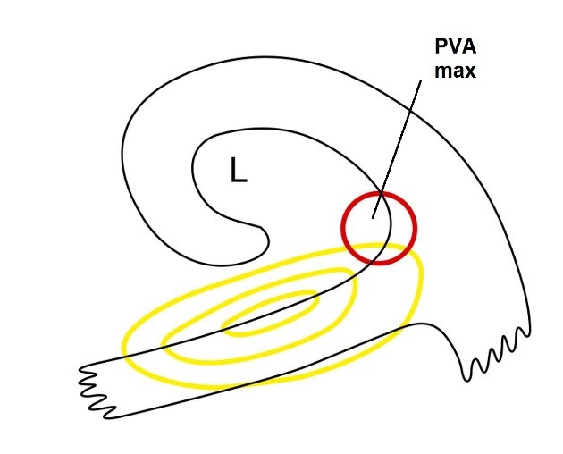
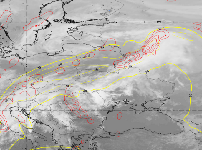
Figure 7:
Left: Schematic of the jet streak positions and the positive vorticity advection maximum (PVA max) at 300 hPa during the mature stage.
Right: IR 10.8 μm imagery from 2 December 2021 at 12:00 UTC. Isotachs at 300 hPa in yellow and PVA at 300 hPa in red. Mean sea level pressure in black.
Key Parameters
The behaviour of the key parameters of the Shapiro-Keyser cyclone will be demonstrated here for the four development stages:
- wave stage
- intensification stage
- mature stage
- dissipation stage
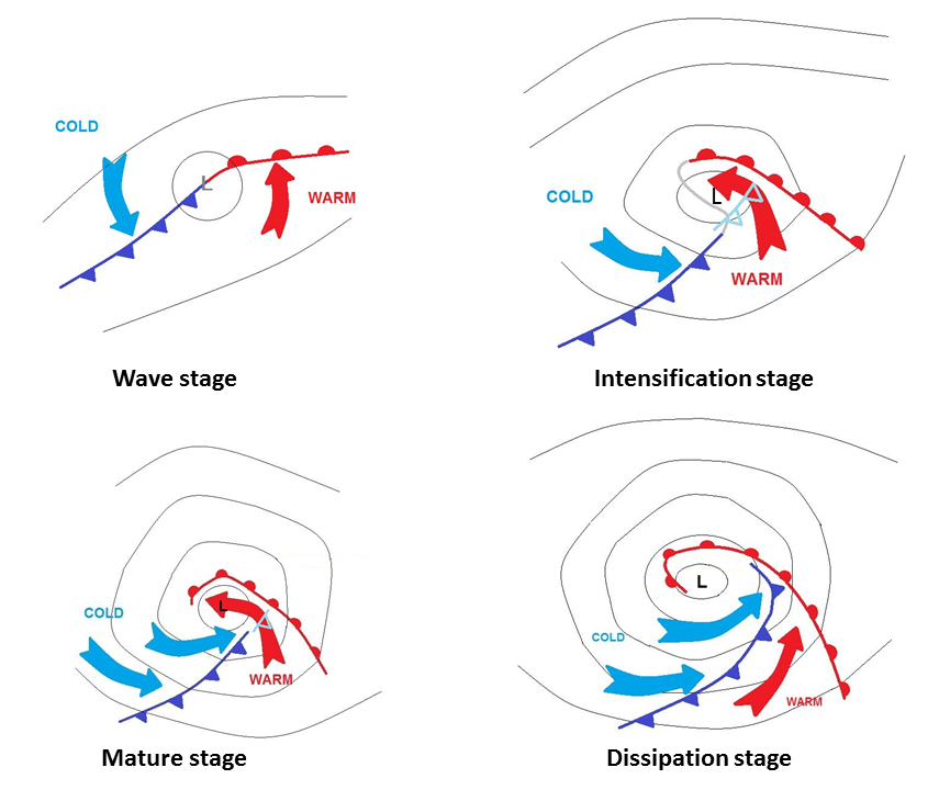
Figure 1: The four developement stages of the Shapiro-Keyser cyclone.
The key parameters chosen here are displayed on pressure levels. The important key parameters are basically the same as those for the Norwegian cyclone type, so we will focus on those key parameters, which follow different behaviour in the Shapiro-Keyser cyclone type. These parameters are:
- the geopotential height at 500 hPa and the mean sea level pressure
- the equivalent potential temperature at 850 hPa
- the temperature advection at 850 hPa
- the humidity at different levels
- the position of the jet and the jet streaks at 300 hPa
A case occurring from 02 to 04 March 2022 is chosen here to illustrate the Shapiro-Keyser cyclone development. It demonstrates the typical behaviour of the selected key parameters and reflects the idealised interaction of NWP parameters with the cloud configuration of a Shapiro-Keyser cyclone.
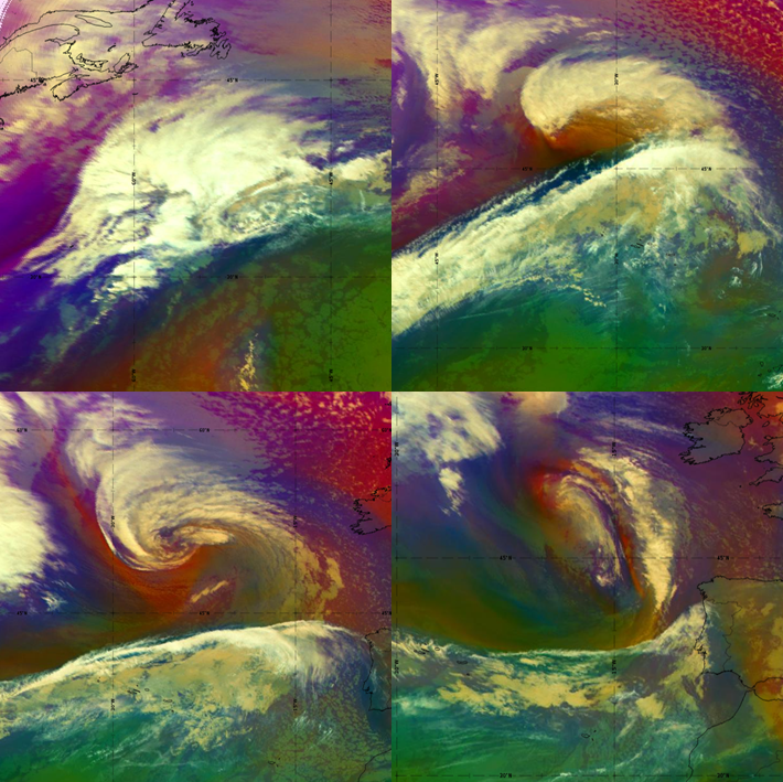
Figure 2: 2 – 4 March 2022, Airmass RGB
U.l. 09:00 UTC on 2 March 2022, Wave stage; u.r.: 18:00 UTC on 3 March 2022, Intensification stage;
l.l. 09:00 UTC on 4 March 2022, Mature stage and l.r. 21:00 UTC on 4 March 2022, Dissipation stage
Typical key parameter features for Shapiro-Keyser cyclogenesis
Geopotential height
- Mean sea-level pressure (or pressure close to the surface):
- At the early cyclogenesis stage, either a weak surface low or a distinct trough is observed. The surface pressure minimum deepens until the cyclone reaches the mature stage and then it starts to weaken.
- 500 hPa geopotential height:
- Shapiro-Keyser cyclone tend to develop in a high-index circulation. This means that the geopotential height in the upper troposphere has a strong zonal component at least during the early development stages.
- In the upper-levels, two phenomena can be observed regarding the geopotential height: the transition from a trough to a closed circulation around a pressure minimum and the shift of the trough axis from west to east during the wave and intensification stages. During the mature stage, the upper-level pressure minimum is superimposed on the surface pressure minimum and moves eastward of the surface pressure minimum during the dissipation stage.
- If we consider an axis that links the pressure minima at different levels, this axis is tilted westward until the cyclone reaches the mature stage (at which it is vertical) and is then tilted eastward in the dissipation phase.

Figure 3: Schematics of geopotential Height at 1000 hPa (black) and 500 hPa (cyan) superimposed on the Airmass RGB.

Figure 4: 2 – 4 March 2022, Airmass RGB, mean sea level pressure (black) and geopotential height at 500 hPa (cyan).
U.l. 09:00 UTC on 2 March 2022, Wave stage; u.r.: 18:00 UTC on 3 March 2022, Intensification stage;
l.l. 09:00 UTC on 4 March 2022, Mature stage; l.r. 21:00 UTC on 4 March 2022, Dissipation stage.
Equivalent potential temperature
- Equivalent potential temperature at 850 hPa:
- This parameter is suited for displaying air mass boundaries as it combines temperature and humidity. Both these quantities typically have high gradients at fronts and air mass boundaries. In the case of a Shapiro-Keyser cyclone, the parameter clearly shows how cold and dry air masses wrap around the warm core of the system until it is completely secluded from the warm sector.
- The frontal zones (i.e., cold and warm fronts) are characterized by higher gradients in the equivalent potential temperature field. A cold frontal fracture is seen in the intensification and mature phases in the region where the cold front would normally join the warm front. In fact, a weaker but inactive frontal zone can be seen connecting the western end of the cold front to the northern tip of the warm front.
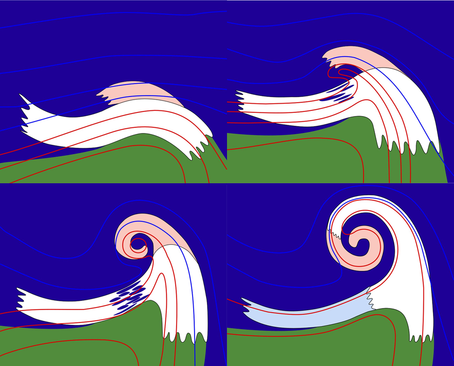
Figure 5: Schematics of the equivalent potential temperature at 850 hPa (red and blue) superimposed on the Airmass RGB.
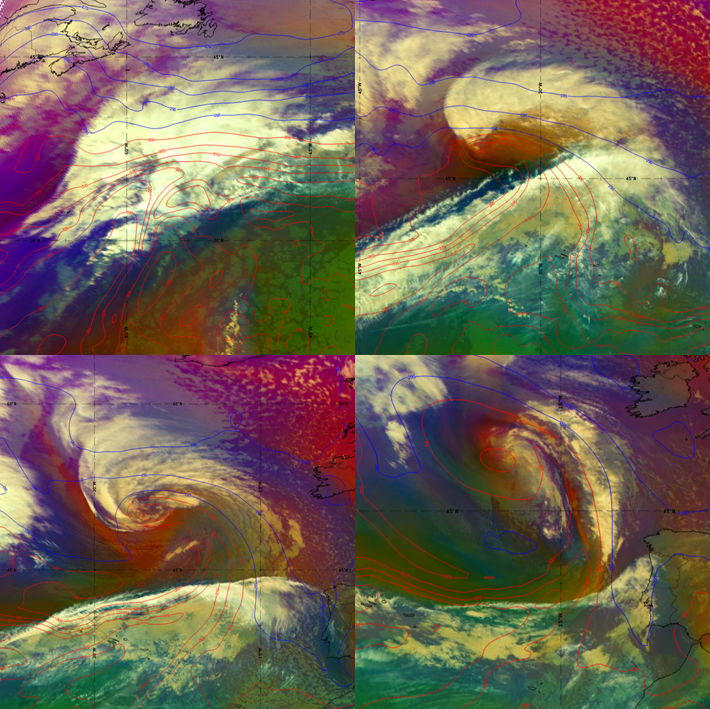
Figure 6: 2 – 4 March 2022, Airmass RGB, equivalent potential temperature at 850 hPa (red and blue).
U.l. 09:00 UTC on 2 March 2022, Wave stage; u.r.: 18:00 UTC on 3 March 2022,
Intensification stage; l.l. 09:00 UTC on 4 March 2022, Mature stage; l.r. 21:00 UTC on 4 March 2022, Dissipation stage.
Temperature advection
- Temperature advection at 850 hPa:
- During the wave stage, we find similar behaviour to that for the Norwegian cyclone type: the cold front is associated with cold air advection (CA) at all-levels on their rear side and so is the warm front with warm air advection (WA).
- The intensification phase is characterized by a dipole of WA and CA, where WA is found at the surface low and CA behind the cold front. This strong dipole at low to middle levels is typical for rapid cyclogenesis.
- During the mature stage, WA prevails behind the warm front that circles around the surface low, while CA coincides with the region where cold air penetrates the area between the cold front and the cyclone centre.
- Finally, weak WA and CA maxima are visible around the cyclone core during the dissipation stage. They are collocated with either the warm front or the dry intrusion, both of which wrap around the warm core.
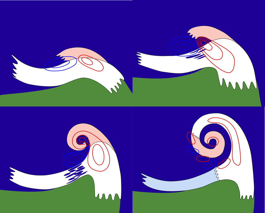
Figure 7: Schematics of the temperature advection at 850 hPa (red, positive and blue, negative) superimposed on the Airmass RGB.

Figure 8: 2 – 4 March 2022, Airmass RGB, temperature advection at 850 hPa (red and blue).
U.l. 09:00 UTC on 2 March 2022, Wave stage; u.r.: 18:00 UTC on 3 March 2022, Intensification stage;
l.l. 09:00 UTC on 4 March 2022, Mature stage; l.r. 21:00 UTC on 4 March 2022, Dissipation stage.
Humidity
- Relative humidity at levels 300 and 700 hPa:
- The warm core separation process is clearly reflected in the humidity fields at all levels. A downward directed stream of dry air is found at the rear side of the cold front. This stream is identical to the dry intrusion conveyor belt.
- This downward propagation of dry air masses is most distinctive during the intensification and mature stages. It is first noticeable at higher levels during the intensification stage and later, at lower levels, during the mature and dissipation stages.
- The downward progression of dry air masses is responsible for the transformation of the upper-level cold front into a cold front that again reaches down to the ground. Due to diabatic heating processes during the downward motion, the temperature gradient at the rebuilt cold front is not very strong. The cold front is characterized mainly by a humidity gradient.
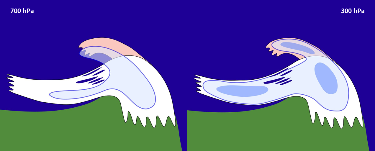
Figure 9: Schematics of relative humidity at 700 and 300 hPa (blue) during the intensification stage superimposed on the Airmass RGB.
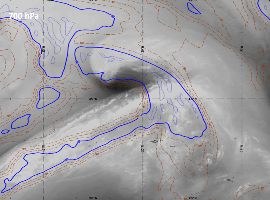
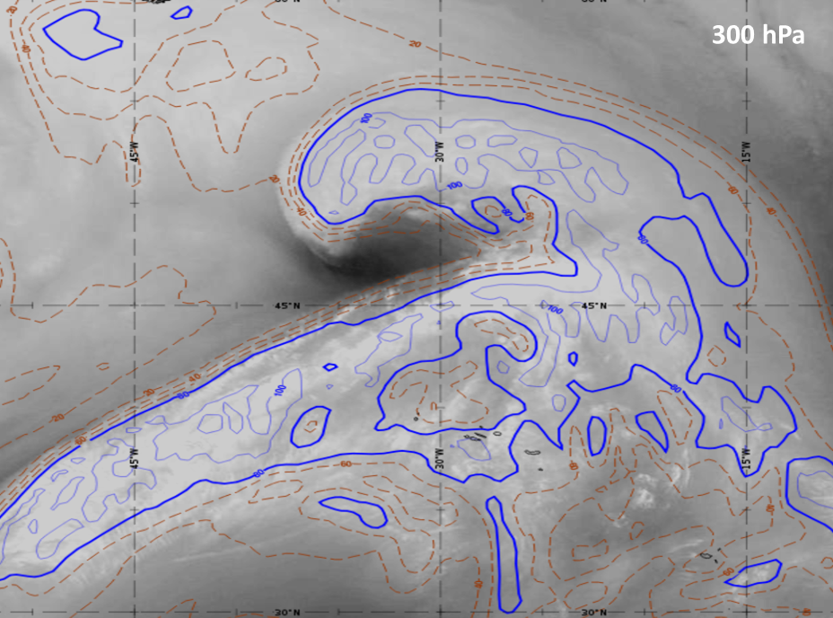
Figure 10: WV6.2 µm – 3 March 2022 at 18:00 UTC, intensification stage. Relative humidity at levels 300 and 700 hPa.
NB: The WV6.2 µm image is not representative for 700 hPa humidity.
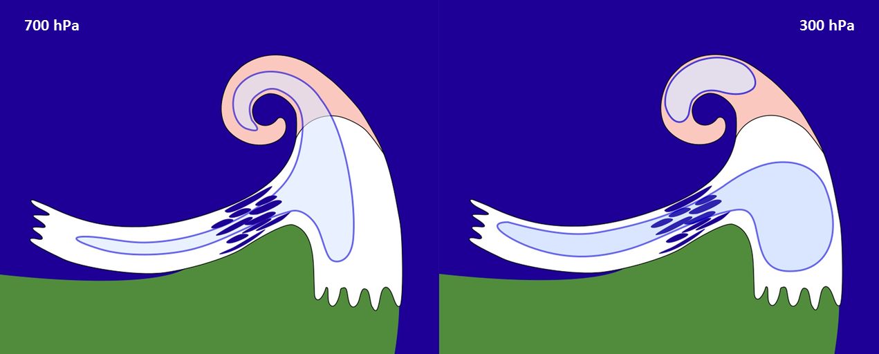
Figure 11: Schematics of relative humidity at 700 and 300 hPa (blue) during the mature stage superimposed on the Airmass RGB.
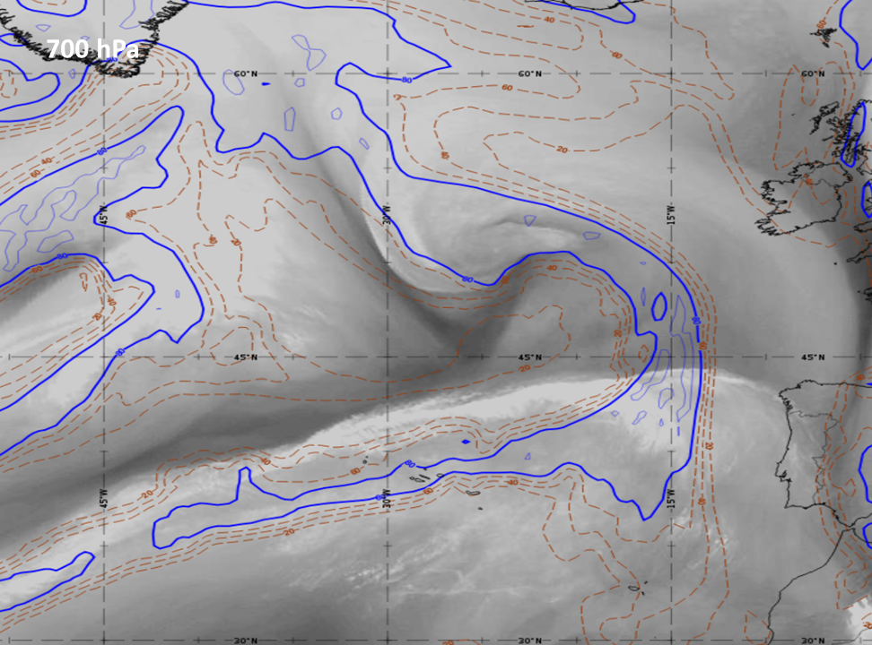

Figure 12: WV6.2 µm – 4 March 2022 at 09:00 UTC, mature stage. Relative humidity at levels 300 and 700 hPa.
NB: The WV6.2 µm image is not representative for 700 hPa humidity.
Wind speed and vorticity advection at jet level
- Isotachs and cyclonic (positive) vorticity advection (CVA) at 300 hPa:
- During the wave stage of a Shapiro-Keyser system, we usually find two jet streaks. They are aligned in such a way that the left exit region of one jet streak is superimposed on the right entrance region of the other. This arrangement is called "jet streak coupling", with the effect that the two CVA maxima collocate, for which reason their impact on surface convergence is increased
- Jet streak coupling is still present during the intensification stage, even though the angle between the jet streaks becomes narrower.
- At the end of the intensification and during the mature stage, the axes of the jets become nearly perpendicular to each other.
- With decreasing meridional temperature gradient, the jets become weaker in the dissipation phase.
- During the later stages, the jet streaks are usually no longer coupled, nor is there an interaction between upper-level divergence and the surface pressure minimum.
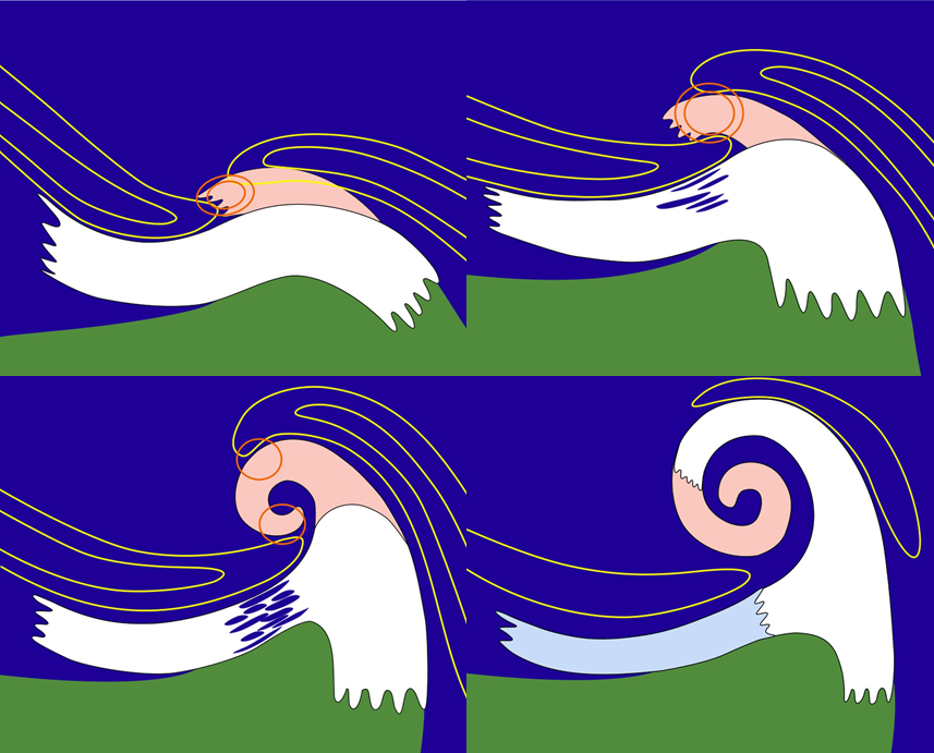
Figure 13: Schematics of the jet streak at 300 hPa (yellow) superimposed on the Airmass RGB. Left exit and right entrance regions are indicated by red circles.
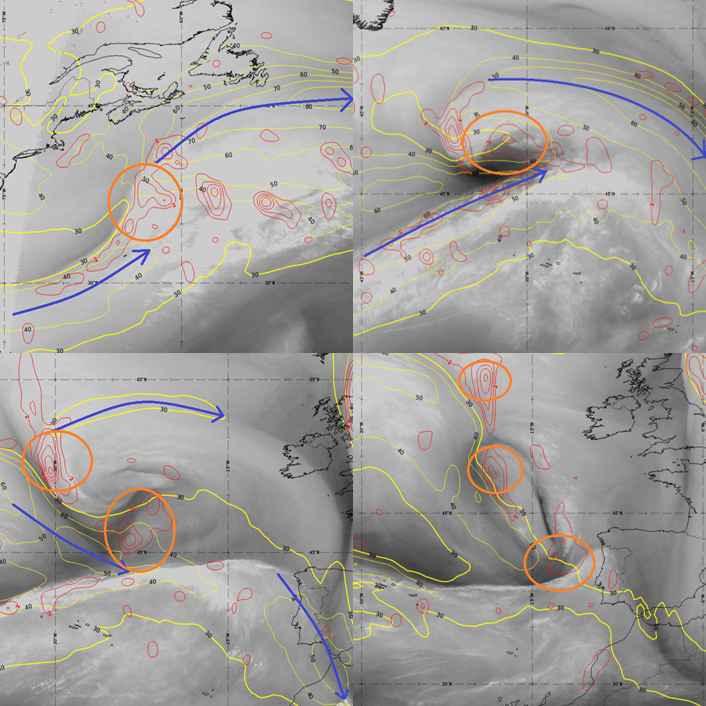
Figure 14: 2 – 4 March 2022, WV 6.2 µm, isotachs (yellow), CVA maxima at 300 hPa (red) and jet axis (blue arrows). CVA maxima in the left exit or in the right entrance region are marked by orange circles.
U.l. 09:00 UTC on 2 March 2022, Wave stage; u.r.: 18:00 UTC on 3 March 2022, Intensification stage;
l.l. 09:00 UTC on 4 March 2022, Mature stage; l.r. 21:00 UTC on 4 March 2022, Dissipation stage.
Typical Appearance In Vertical Cross Sections
From the wave stage on, the vertical structure of Shapiro-Keyser cyclones differs fundamentally from the Norwegian cyclone type. This can be seen in vertical cross sections through the fronts of the Shapiro-Keyser cyclone using NWP model data. As in the previous chapters, we focus on the phases where the warm air intrusion forms, i.e. the intensification stage until the final stage of the life cycle: the dissipation stage.
The model parameters that best characterize the evolution of the Shapiro-Keyser cyclone in vertical cross sections (VCS) are:
- temperature
- temperature advection and
- humidity
The Shapiro-Keyser cyclone development case study used here to demonstrate typical vertical cross-sections (using ECMWF model data) is from 3 March 2022 at 15:00 UTC for the intensification stage, 4 March 2022 at 12:00 UTC for the mature stage and 4 March 2022 at 21:00 UTC for the dissipation stage.
The intensification stage
During the intensification stage, warm air from the warm sector of the system invades the area of the surface low at low to middle levels of the troposphere. The protruding warm air masses are separated from the polar air by a baroclinic zone that gradually adopts the characteristics of a warm front. At the same time, the upper-level cold front remains aligned to the lower-level cold front.
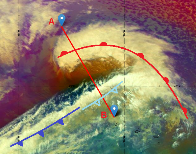

Figure 1:
Left: Airmass RGB from 3 March 2022 at 15:00 UTC with fronts and the position of the vertical cross section.
Right: Schematic of the intensification stage of the Shapiro-Keyser cyclone with fronts and the position of the vertical cross section.
At the intensification stage, the warm front (red line) is very distinctive in the VCS. The warm core and the warm sector consist of a uniform air mass; there is no temperature or humidity gradient below 700 hPa. Nevertheless, at higher levels, an upper-level cold front (light blue line) that corresponds to a weak temperature gradient and a stronger humidity gradient (Figure 4) is clearly seen.

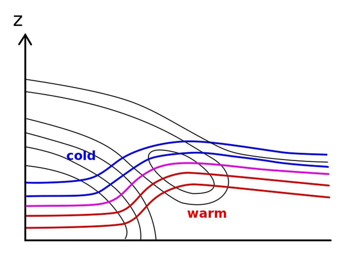
Figure 2:
Left: Vertical cross section showing the equivalent potential temperature (black lines) and the temperature from ECMWF model data (dotted red and blue lines).
Right: Schematic of the vertical cross section.
The VCS shows pronounced warm air advection within the warm front and moderate cold air advection within the upper-level cold front. This confirms that the latter is mainly characterized by a humidity rather than by a temperature gradient.
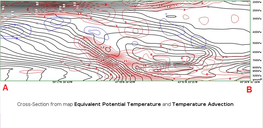
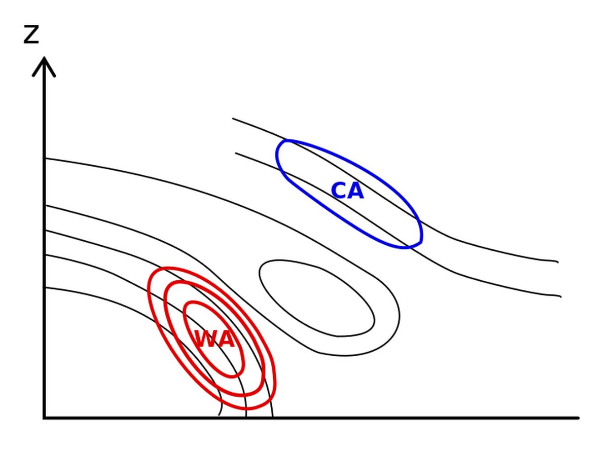
Figure 3:
Left:Vertical cross section showing the equivalent potential temperature (black lines) and the temperature advection (red and blue lines) from ECMWF model data.
Right: Schematic of the vertical cross section.
The dry intrusion between the warm front and the upper-level cold front is clearly visible in the VCS. During the intensification stage, the dry intrusion affects the mid- and upper troposphere only.
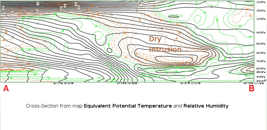
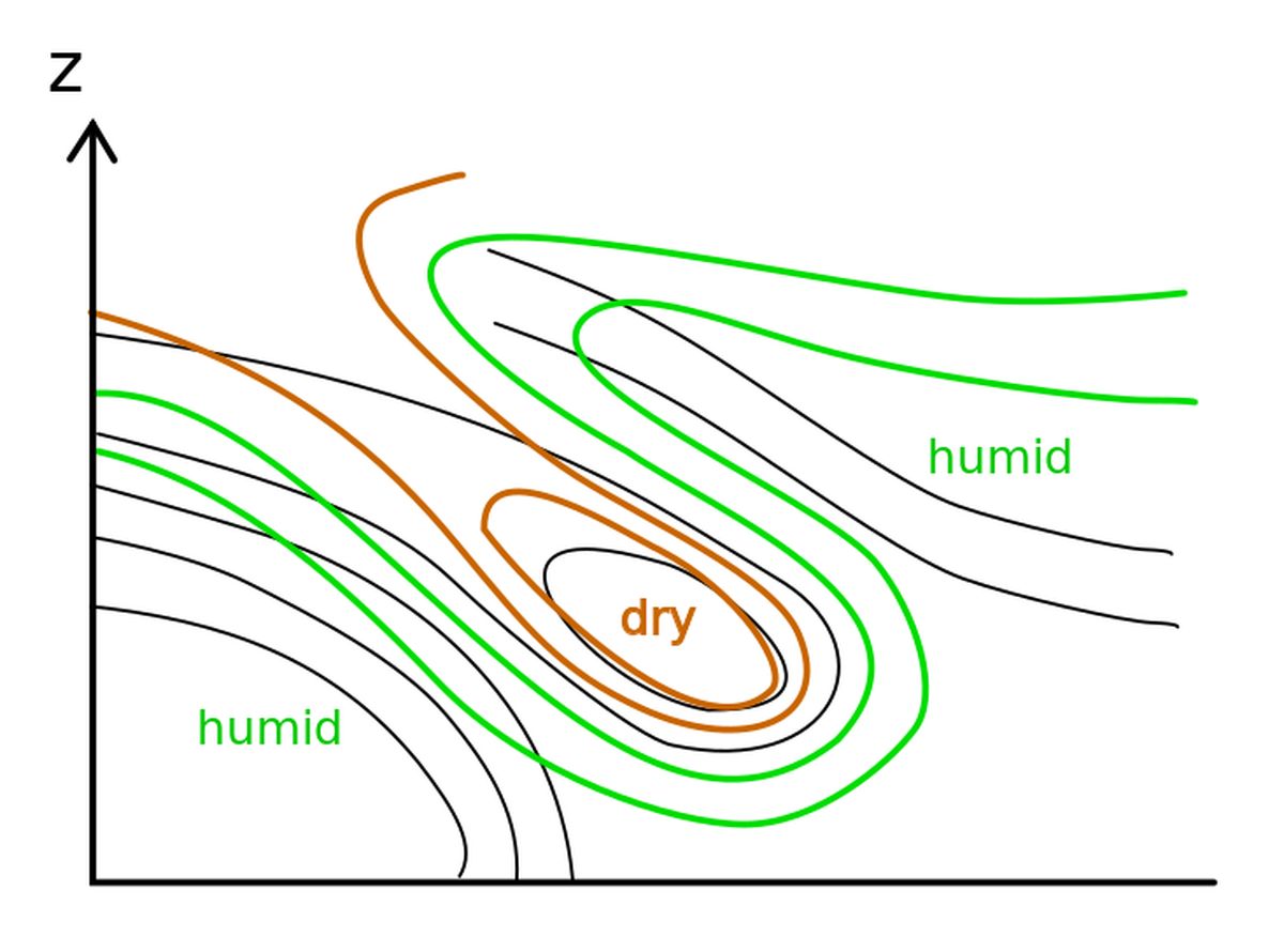
Figure 4:
Left:Vertical cross section showing the equivalent potential temperature (black lines) and relative humidity (green and brown lines) from ECMWF model data.
Right: Schematic of the vertical cross section.
The mature stage
During the mature stage, the warm core of the Shapiro-Keyser system becomes secluded from the warm sector. A VCS through the warm core and the cold front of the Shapiro-Keyser system shows a complex pattern of successive fronts depending on how far the seclusion has progressed.
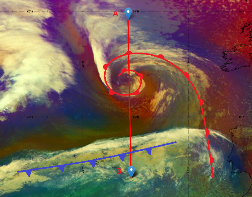

Figure 5:
Left: Airmass RGB from 4 March 2022 at 12:00 UTC with fronts and the position of the vertical cross section.
Right: Schematic of the mature stage of the Shapiro-Keyser cyclone with surface fronts and the position of the vertical cross section.
The number of warm fronts (red lines in Figure 6) depicted in the VCS depends on how far warm air seclusion has progressed. During the seclusion process, cold air wraps around the warm core that is very distinct in the vertical temperature chart. At this stage, the upper-level cold front has transformed into a surface front (blue line), which is characterized by a strong humidity gradient rather than by a temperature gradient.

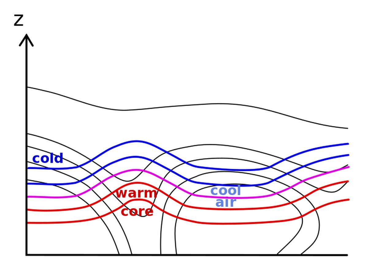
Figure 6:
Left: Vertical cross section showing the equivalent potential temperature (black lines) and the temperature from ECMWF model data (dotted red and blue lines).
Right: Schematic of the vertical cross section.
The warm fronts located around the warm core are characterized by warm air advection and the cold front by cold air advection.

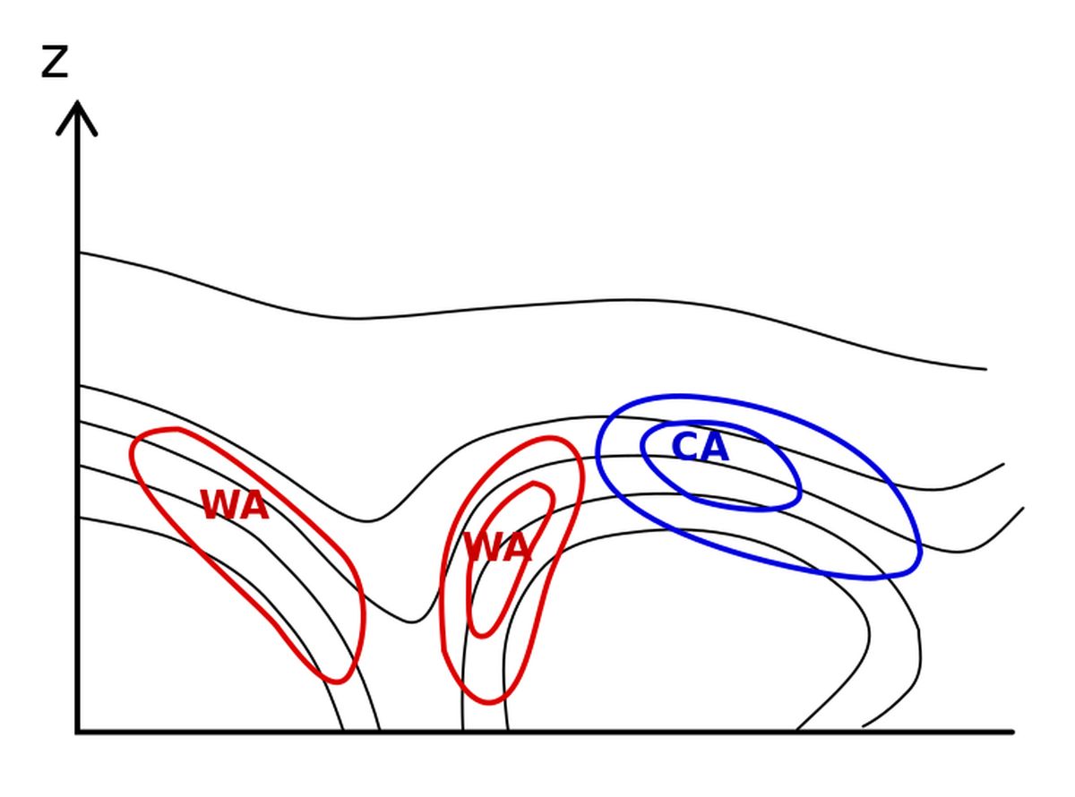
Figure 7:
Left: Vertical cross section showing the equivalent potential temperature (black lines) and the temperature advection (red and blue lines) from ECMWF model data.
Right: Schematic of the vertical cross section.
Figure 8 shows how the dry intrusion has affected even lower atmospheric regions than in the intensification stage.
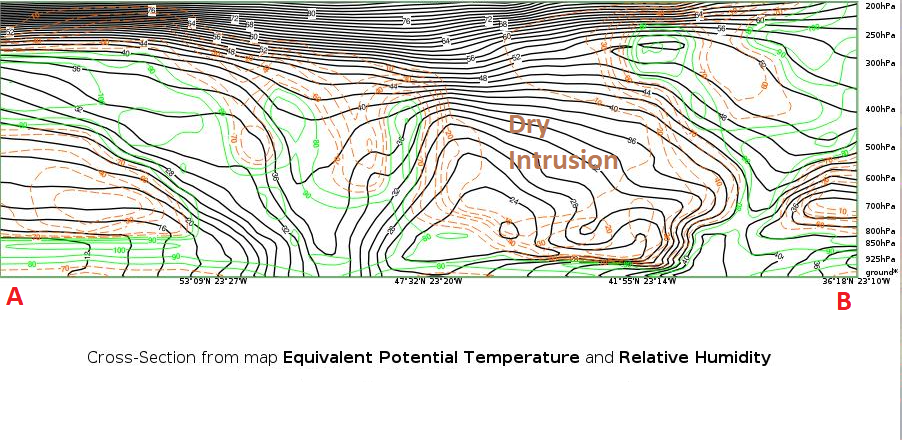
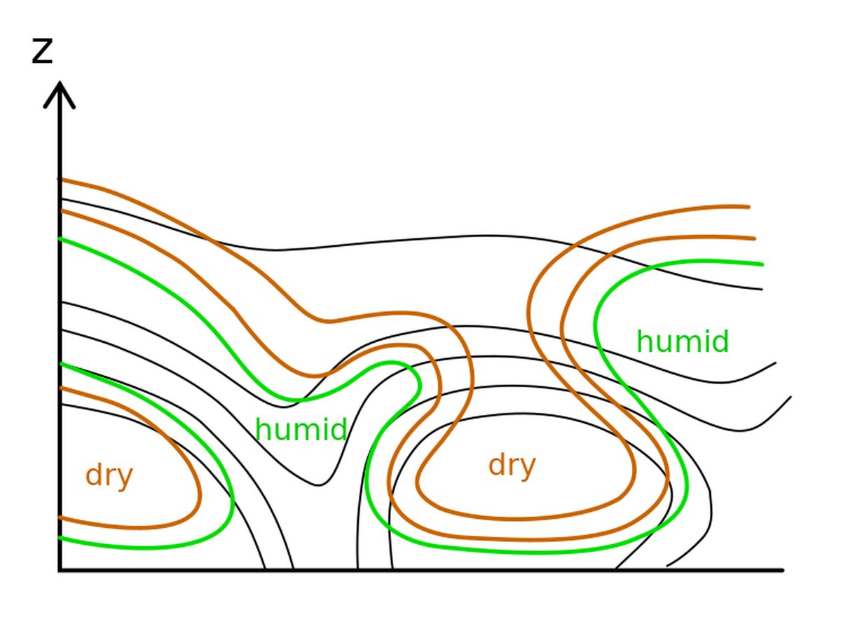
Figure 8:
Left:: Vertical cross section showing the equivalent potential temperature (black lines) and relative humidity (green and brown lines) from ECMWF model data.
Right: Schematic Schematic of the vertical cross section.
The dissipation stage
During the final part of the Shapiro-Keyser cyclone life cycle, the temperatures of the warm core and the surrounding cold air masses adjust, so that the warm front weakens. The cold front finally catches up with the warm front, a similar process to that of the Norwegian cyclone type.

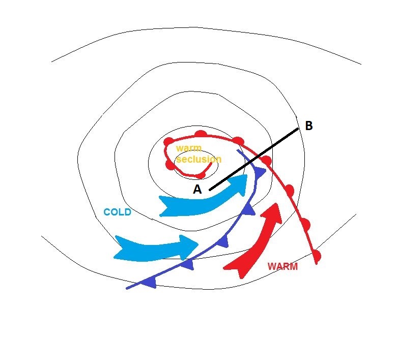
Figure 9:
Left: Airmass RGB from 4 March 2022 at 21:00 UTC with fronts and the position of the vertical cross section.
Right: Schematic of the dissipation stage of the Shapiro-Keyser cyclone with surface fronts and the position of the vertical cross section.
The VCS through the cold and warm front shows them forming a V-shape when looking at equivalent potential temperature. The occlusion is of the warm front type, as the cold front does not reach the ground. The cold front is primarily characterized by a strong humidity gradient rather than by a temperature gradient (see Figure 10).

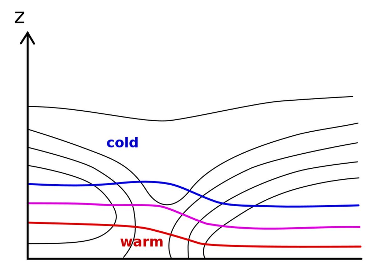
Figure 10:
Left:: Vertical cross section showing equivalent potential temperature (black lines) and temperature (dotted red and blue lines) from ECMWF model data.
Right: Schematic of the vertical cross section.
The warm front is characterized by warm air advection. The magnitude depends on the propagation speed and the intensity of the temperature gradient.

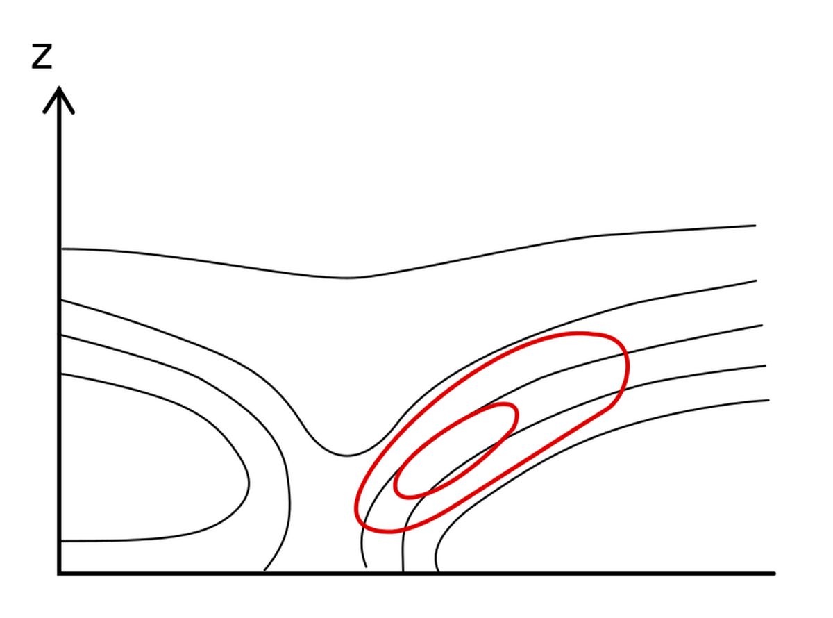
Figure 11:
Left: Vertical cross section showing the equivalent potential temperature (black lines) and temperature advection (red and blue lines) from ECMWF model data.
Right: Schematic of the vertical cross section.
Higher moisture content and temperatures are found in the narrowing warm sector between the cold and the warm front. This frontal configuration is the same as in the Norwegian cyclone type where it is called an occlusion.

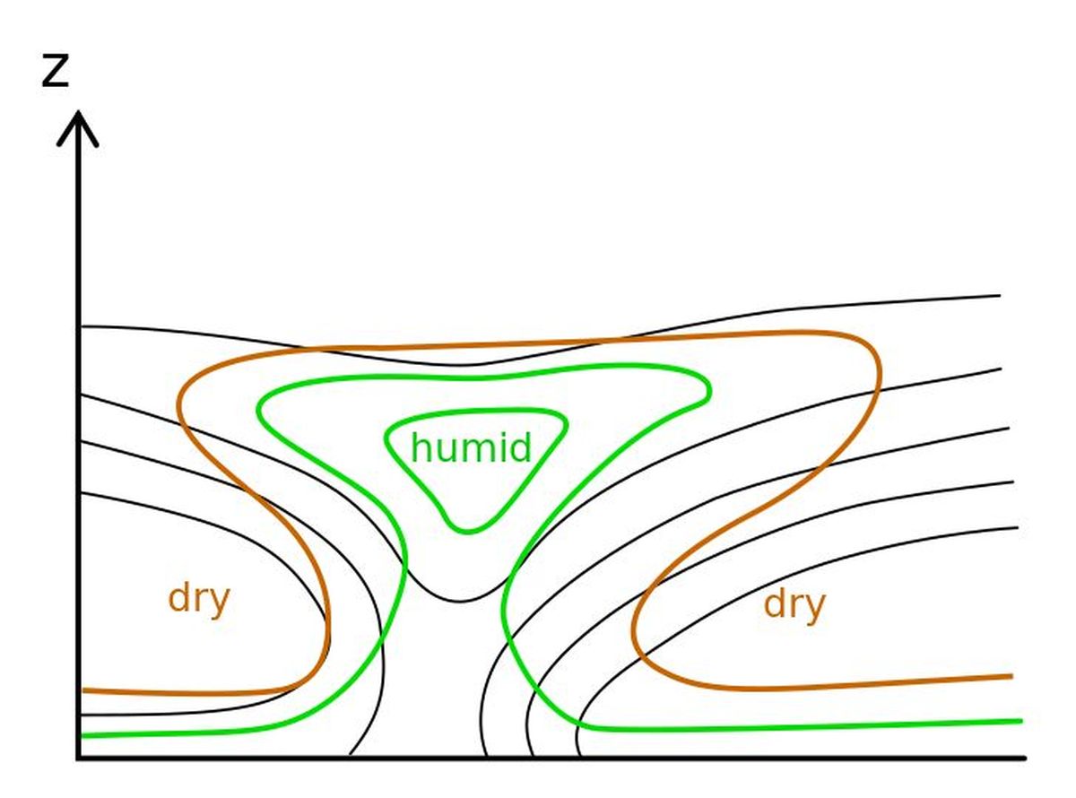
Figure 12:
Left: Vertical cross section showing equivalent potential temperature (black lines) and relative humidity (green and brown lines) from ECMWF model data.
Right: Schematic of the vertical cross section.
Weather Events
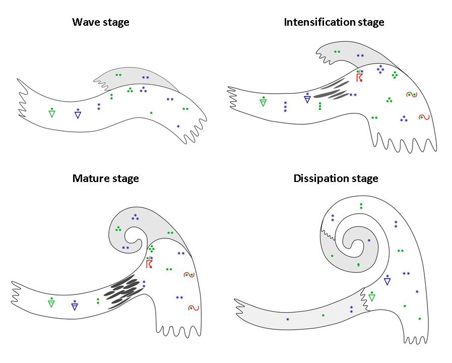
Figure 1: The most frequent weather events occurring during the four evolution stages of a Shapiro-Keyser cyclone.
| Parameter | Description |
|---|---|
| Precipication | Most intense precipitation occurs during the intensification and the mature stage. The highest precipitation rates occur in the area of the rising warm conveyor belt (e.g., warm front). At advanced stages and with the splitting of the warm conveyor belt into two branches, higher precipitation rates occur inside the occlusion-like cloud band. |
| Temperature | Warm air masses occur in the warm sector and within the system core (i.e., surface pressure minimum). A temperature drop occurs after the passage of the cold front. |
| Wind (incl. gusts) | High wind speeds occur, related to the passage of the cold front and gusty winds behind the cold front. The highest wind speeds occur at the southern tip of the occlusion-like cloud band (e.g., Sting Jet). |
| Other relevant information | Turbulence may occur at jet-level near the tropopause fold. There is a risk of freezing rain below the warm front in winter. Thunderstorms embedded in the cold front may also be encountered in winter. |
Weather events for the early stages of the Shapiro Keyser cyclone are described in detail in the chapter related tI uso the conceptual model "Wave" which reflects the early stage of a Shapiro-Keyser cyclone. We therefore start with the intensification stage, followed by the mature and dissipation stages. A Shapiro-Keyser cyclone development that lasted from 30 November at 18:00 UTC to 02 December 2021 at 00:00 UTC is used as a case-study for illustration.
The intensification stage (30 November 2021 at 18:00 UTC):
Most intense precipitation is found at the western part of the warm front (Ireland and Scotland). This area is collocated with the right entrance region of a jet streak.
|
|
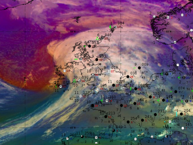
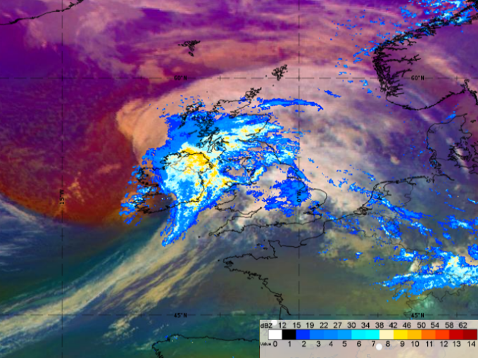
Figure 2: Airmass RGB with Synop data and with superimposed Radar reflectivity (move the slider to compare the two images).
The NWC SAF satellite products Precipitating Clouds (PC) and Convective Rainfall Rate (CRR) show highest probabilities for rain and highest hourly rainfall rates within the warm front and the warm sector.
|
|
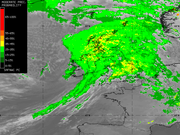
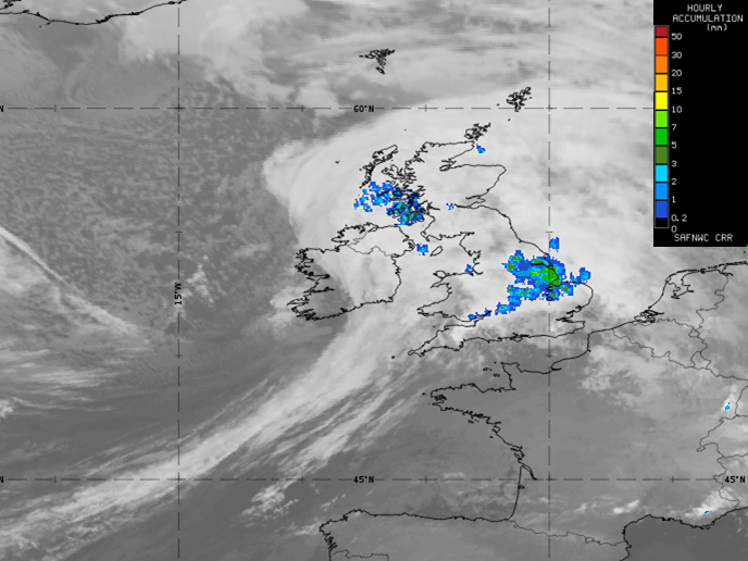
Figure 3: : NWC SAF products Precipitating Clouds and Convective Rainfall Rate (move the slider to compare the two images).
The mature stage (1 December 2021 at 12:00 UTC):
Intense showers partly occur along the cold front where the cloud structure is more inhomogeneous. A more continuous type of rain in the warm front parts of the system characterizes the precipitation that occurs during the mature stage of a Shapiro-Keyser cyclone.
|
|
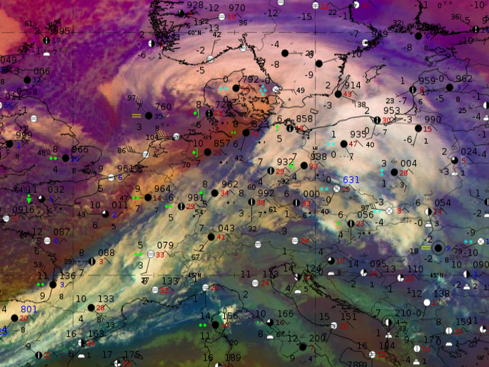
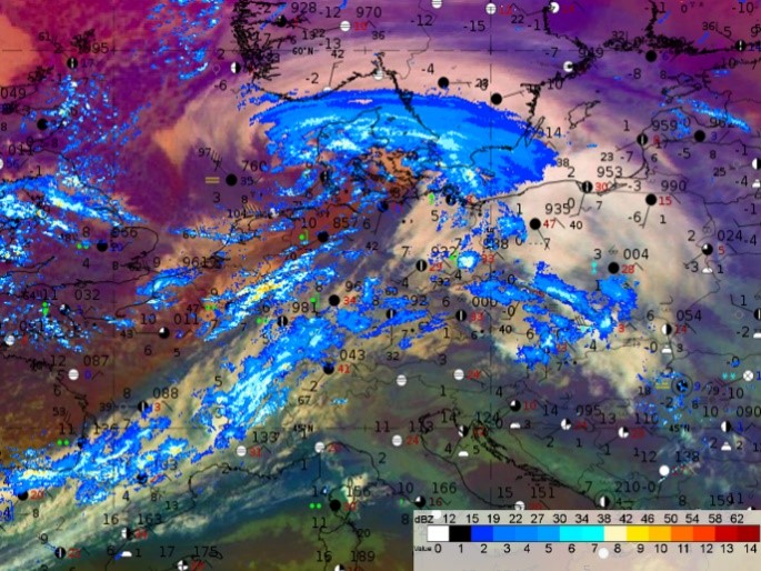
Figure 4: : Airmass RGB with Synop data and with superimposed Radar reflectivity (move the slider to compare the two images).
Both NWC SAF precipitation products show widespread rainfall in the warm front areas of the Shapiro-Keyser system. Locally, precipitation can be more intense within the cold front
|
|
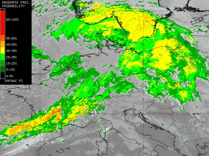
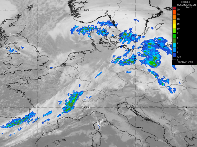
Figure 5: : NWC SAF products Precipitating Clouds and Convective Rainfall Rate (move the slider to compare the two images)
The dissipation stage (2 December 2021 at 00:00 UTC):
At the end of the cyclones life cycle, most precipitation occurs within the system core and the warm front. Showers may still occur in the cold front section of the system.
|
|
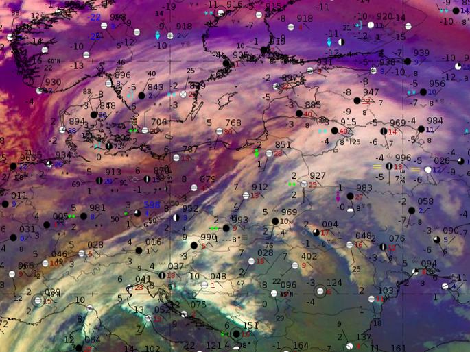
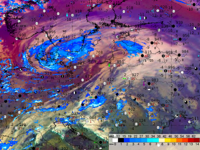
Figure 6: : Airmass RGB with Synop data and with superimposed Radar reflectivity (move the slider to compare the two images).
While the PC product shows higher precipitation probabilities at the warm front of the decaying system, the CRR product hardly shows any precipitation spots.
|
|
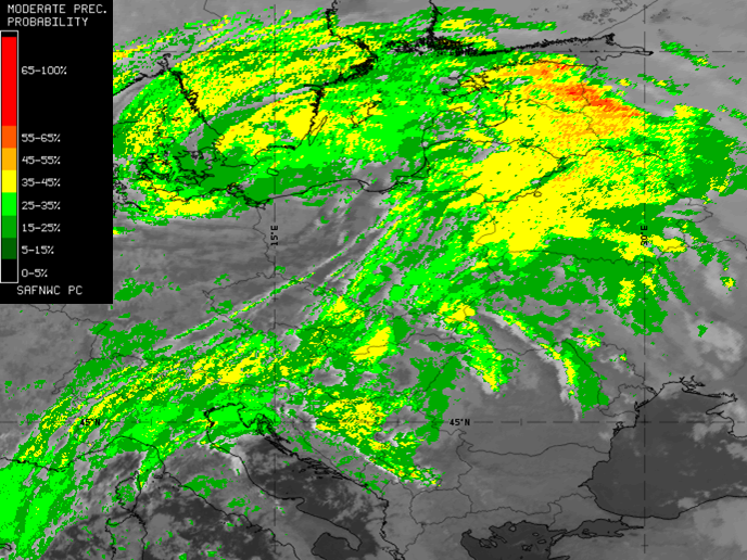
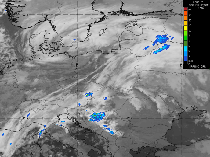
Figure 7: NWC SAF products Precipitating Clouds and Convective Rainfall Rate (move the slider to compare the two images).