Table of Contents
Cloud Structure In Satellite Images
The term Baroclinic Boundary is used to describe a front like cloud band, which is oriented differently compared with those associated with an actual front. It can also be distinguished from stationary fronts and air mass boundaries. A Baroclinic Boundary does not propagate significantly. An investigation was carried out on 60 cases.
The investigation showed Baroclinic Boundaries at several typical locations (e.g. indicated by the height field at 500 hPa):
- At the rear of a synoptic scale trough (most frequent type, about 58 cases, schematic below left)
- Baroclinic Boundary associated with an Upper Level Low (6 cases, schematic below middle)
- Baroclinic Boundary associated with a deformation zone at a saddle point in the upper height fields (3 cases, schematic below right)
|
|

|
Appearance in the basic channels
- IR imagery:
- Dark to light grey low and mid-level cloud band
- The Baroclinic Boundary usually appears darker (i.e. warmer cloud tops) than frontal cloud
- Sometimes a bright jet cloud fibre forms or fibrous clouds are embedded within the cloudband
- WV imagery:
- The Baroclinic Boundary appears as a dark grey to grey cloud band sometimes with bright high fibres embedded
- The Baroclinic Boundary generally appears weaker in WV than a frontal cloud band
- VIS imagery:
- Depending on the type of cloud the VIS image shows low white patches or cloud bands. If they exist, thin high cloud fibres appear grey.
Appearance in the basic RGBs:
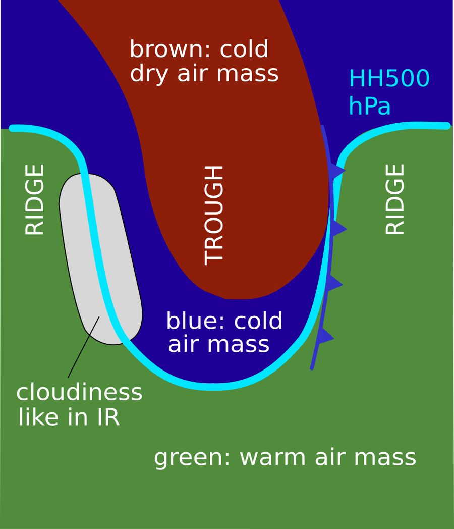
Airmass RGB
In the Airmass RGB there are usually blue to brown colours in front of the baroclinic boundary (the cyclonic side), representing the airmasses in the upper level trough area, and greenish colours in the warm sector of the subsequent frontal system representing the warm air.
The cloud band itself appears very similar to that in the IR image.
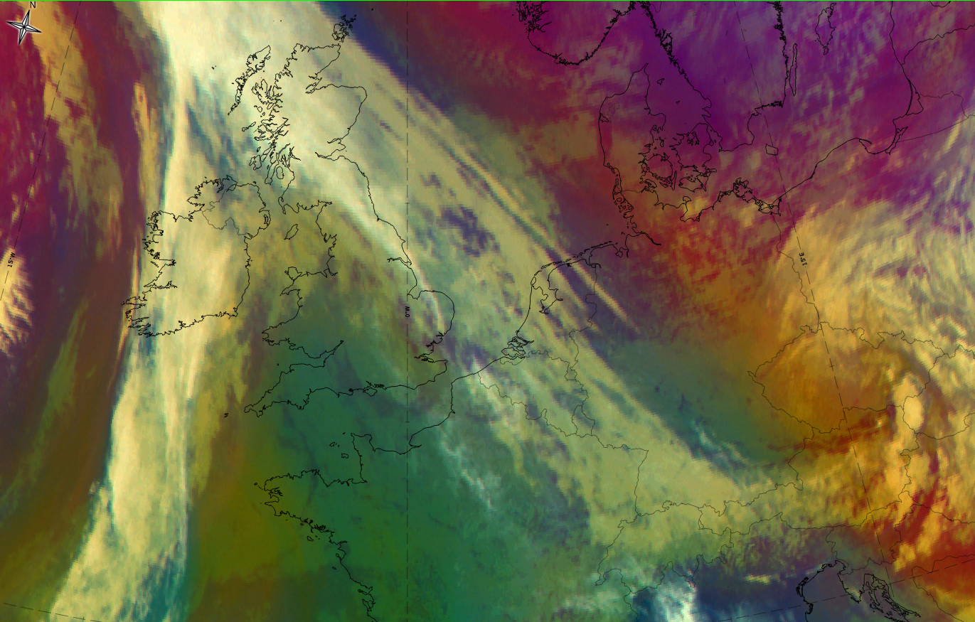
Dust RGB
In the Dust RGB there are blue to pinkish blue colours on both sides of the baroclinic cloud band where there are cloud free areas; often cloud systems are often included and these appear mostly as ochre colours representing low to mid-level cloud.
The cloud band of the baroclinic boundary has mostly yellowish to ochre colours, typical for mid-level cloud, and some dark red to black stripes and patches where there are thicker and/or higher cloud fibres above the mid-level cloud. Black fibres can also occur, mostly at the cloud edges, representing high translucent cloud fibres.
 |
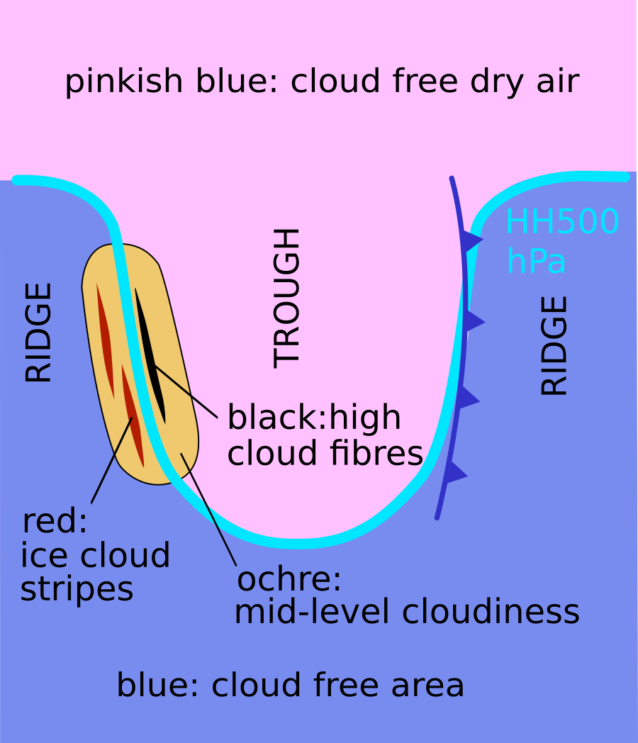 |
Basic RGB schematics. Left: Airmass RGB; Right: Dust RGB.
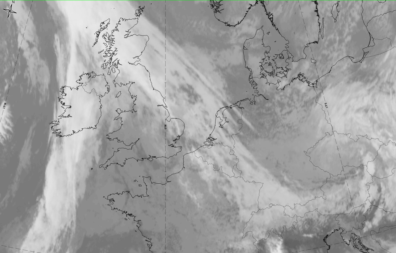
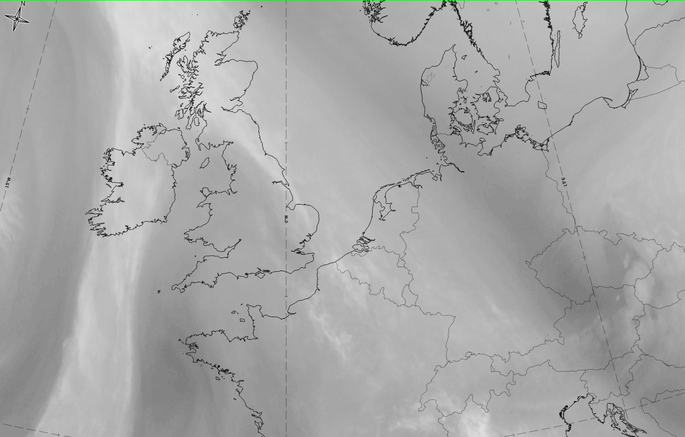
The case from 5 October 2019 at 12UTC is a good example of a baroclinic boundary cloud band at the rear side of an upper level trough. It extends from the North Sea across the Netherlands to the western Alps.
|
|
|
|

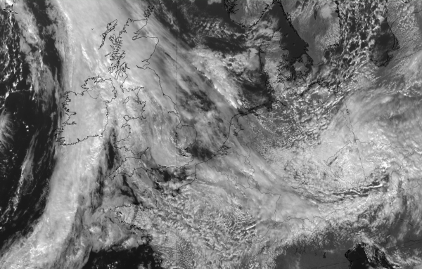

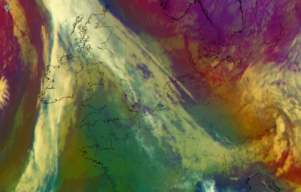
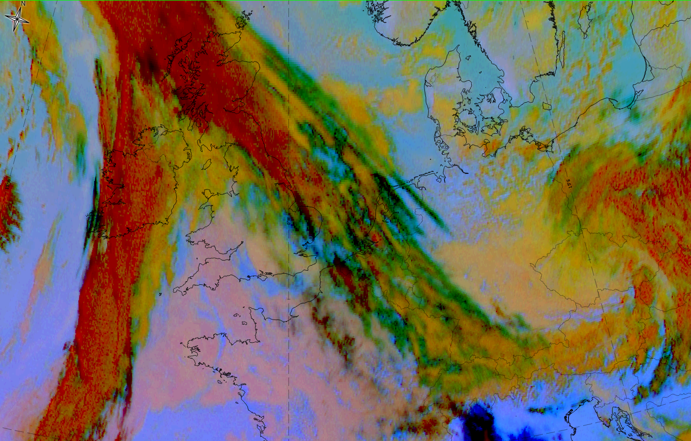
5 October 2019, 12 UTC: 1st row: IR (above)+ HRV (below); 2nd row: WV above) + Airmass RGB (below); 3rd row: Dust RGB + image gallery
*Note: click on the Dust RGB image to access image gallery (navigate using arrows on keyboard)
| IR | Grey colours with partly fibrous structure. |
| HRV | Some grey cloud patches bust mostly cloud fibres. |
| WV | Grey band of high humidity with some brighter cloud fibres. |
| Airmass RGB | Brown colours to the NE, representing the cold dry air in the trough in front of the baroclinic boundary; bluish colours around the cloud band and greenish colours representing warm air in the warm sector at the rear of the baroclinic boundary. |
| Dust RGB | Ochre colours for low and mid-level clouds, black stripes for high translucent cloud fibres and green colours for thin medium and/or low level cloud. |
Meteorological Physical Background
Baroclinicity, in general, is defined as the state of the atmosphere in which surfaces of constant pressure are intersected by surfaces of constant temperature or constant density. The number, per unit area, of isobaric - isosteric solenoids intersecting a given surface is then a measure of the baroclinicity. High baroclinicity shows up as a high gradient of density or temperature which usually accompanies a change of air mass. Consequently a Baroclinic Boundary is - like a front - in principal a boundary between two different air masses. High gradients of ThetaE and equivalent thickness are parameters which indicate baroclinicity. Baroclinic Boundaries show no significant propagation and their position within the synoptic system is different from a classic front.
From the classic front theory a flow from the warm side associated with a ridge of height contours and a cold flow from the rear side of a trough result in significant confluence within the area of the Baroclinic Boundary. Both are indicated by the wind fields and the relative streams.
The dominating physical process from the colder side - the trough side - will be a relative stream at low and middle levels (see schematic below). At upper levels the Warm Conveyor Belt is dominating, which originates within the ridge (or warm side). Elongation and deformation are also well reflected in the wind fields.
In general, a sinking motion at low levels and rising at middle and upper levels can be observed. The advection of cold, dry air at low levels causes superadiabatic stratification above relatively warmer surfaces. Anyway, the vertical expansion of the cold air mass is less than within a CF. Both characteristics can often be seen in the vertical cross sections (see Typical appearance in vertical cross section). The difference in the vertical extension of the cold air may be connected with the difference in propagation between Cold Fronts and Baroclinic Boundaries.
The typical distribution of relative streams for a frontal system is described here. The schematic below shows the typical distribution of the relative streams of a Baroclinic Boundary. The pattern is valid for all three types of the Baroclinic Boundary.
|
The distribution of vertical streams is similar to a CF in CA. But the sinking of cold air at low levels seems to be contradictory considering the formation of low and middle level cloudiness within the Baroclinic Boundary. One possible explanation may be that the cloudiness forms mainly through condensation at the Boundary between warm and cold air masses, indicated by the slantwise crowding of the isentropes. The sinking at low levels and the rising at upper levels is then compensated by a distinct confluence from different height levels, which is also reflected in the wind fields and the relative streams.
The Baroclinic Boundary to the rear of a synoptic scale trough is the most frequent type and will be therefore be considered as an example in this chapter:
|
19 October 2002/06.00 UTC - Meteosat IR image; position of vertical cross section indicated
|
19 October 2002/06.00 UTC - Vertical cross section; black: isentropes (ThetaE), orange thin: IR pixel values, orange thick: WV pixel values
|

|

|
The left IR image above shows the first type of a Baroclinic Boundary to the rear of an upper level trough. It reaches from the Bay of Biscay to the Tyrrhenian Sea. The image displays a homogenous grey cloud band with high bright fibre clouds at the rear side, indicating a significant jet streak at the rear of the trough. The white line indicates the orientation of the vertical cross section seen in the image above right. In the cross section the superadiabatic stratification at low levels clearly appears more shallow than in a CF. The high gradient of equivalent potential temperature at mid levels indicates the baroclinic zone of the boundary between both air masses.
The set of images below shows the relative streams at 302K, 314K and 320K. The low levels are dominated by sinking diffluent streamlines, showing an intrusion of cold air from the trough, which leads to rather low (warm) cloud tops. At 314K the upper relative streams and the Warm Conveyor Belt result in the limiting streamline in the centre of the cloud band. Both streams are rising weakly. At 320K a rising Warm Conveyor Belt, originating from the ridge dominates the boundary.
|
19 October 2002/06.00 UTC - Meteosat IR image; magenta: relative streams 302K - system velocity: 250° 9 m/s, yellow: isobars
|
19 October 2002/06.00 UTC - Meteosat IR image; magenta: relative streams 314K - system velocity: 250° 9 m/s, yellow: isobars
|
|
|
|
|
|
19 October 2002/06.00 UTC - Meteosat IR image; magenta: relative streams 320K - system velocity: 250° 9 m/s, yellow: isobars
|
In all types of Baroclinic Boundaries the relative streams are, in general, similar to those within Cold Fronts. The most striking difference is the location of the Baroclinic Boundary, which results in an inverted orientation of the relative streams, when compared to a CF.
The crowding of isentropes is an indication of high baroclinicity, both in fronts and in the Baroclinic Boundary. Because of frontal propagation the decline of the isentropes is steep within fronts. In contrast, Baroclinic Boundaries show a more flat decline, which can also be a result of their stationarity.
Key Parameters
- Height contours at 500 hPa:
- Distribution of height at 500 hPa indicates boundary between closed synoptic systems:
- To the rear of a trough
- To the rear and in front of an ULL, in the tear - off stage of development
- At the deformation zone between two troughs and two ridges
- Equivalent thickness:
- A distinct gradient of equivalent thickness accompanies the cloud band
- Mostly weaker than "classical" fronts
- The appearance of this parameter is similar within all 3 types of Baroclinic Boundary
- Thermal front parameter (TFP):
- Maximum of TFP associated with the cloud band
- Normally, weaker than "classical" fronts
- No significant propagation
- The appearance of this parameter is similar within all 3 types of Baroclinic Boundary
Height contours at 500 hPa
- At the rear of synoptic scale trough
- Baroclinic boundary associated with ULL
- Baroclinic Boundary associated with deformation zone at a saddle point of upper height Fields
|
19 October 2002/06.00 UTC - Meteosat IR image; cyan: height contours 500 hPa
|
|
|
|
|
05 February 2002/06.00 UTC - Meteosat IR image; cyan: height contours 500 hPa
|
|
|
|
|
04 April 2002/06.00 UTC - Meteosat IR image; cyan: height contours 500 hPa
|
|
|
|
|
Thermal front parameter (TFP) and equivalent thickness
|
29 November 2002/12.00 UTC - Meteosat IR image; blue: thermal front parameter (TFP) 500/850 hPa, green: equivalent thickness 500/850 hPa
|
|
|
|
Typical Appearance In Vertical Cross Sections
A crowding of isentropes indicates an air mass boundary and a baroclinic zone. Though similar to fronts, the cloud band of the Baroclinic Boundary shows no front like appearance in a vertical cross section. The appearance is similar throughout all types of Baroclinic Boundary.
- Isentropes (equivalent potential temperature):
- Zone of high gradient of equivalent potential temperature, gradient mostly weaker than in fronts
- Flat decline of crowded isentropes - a distinct difference from a front
- Superadiabatic stratification only at low levels (associated with diabatic heating or cold air advection)
- Divergence:
- Zone of convergence within the highest gradient of isentropes, usually weaker than within a frontal zone
- Vertical motion (Omega):
- Upward motion within the gradient zone indicating ascent, but usually weaker than in a frontal zone
- All cases show weak ascent at middle levels
|
19 October 2002/06.00 UTC - Meteosat IR image; position of vertical cross section indicated
|
|
|
|
Isentropes (equivalent potential temperature)
|
19 October 2002/06.00 UTC - Vertical cross section; black: isentropes (ThetaE), orange thin: IR pixel values, orange thick: WV pixel values
|
|
|
|
Divergence
|
19 October 2002/06.00 UTC - Vertical cross section; black: isentropes (ThetaE), magenta thin: divergence, magenta thick: convergence, orange thin: IR pixel values, orange thick: WV pixel values
|
|
|
|
Vertical motion (Omega)
|
19 October 2002/06.00 UTC - Vertical cross section; black: isentropes (ThetaE), cyan thick: vertical motion (omega) - upward motion, cyan thin: vertical motion (omega) - downward motion, orange thin: IR pixel values, orange thick: WV pixel values
|
|
|
|
Weather Events
In general observed precipitation is significantly weaker than in fronts; or there may be no precipitation at all.
| Parameter | Description |
| Precipitation |
|
| Temperature | No connection (stationary) |
| Wind (incl. gusts) | No connection (stationary) |
| Other relevant information |
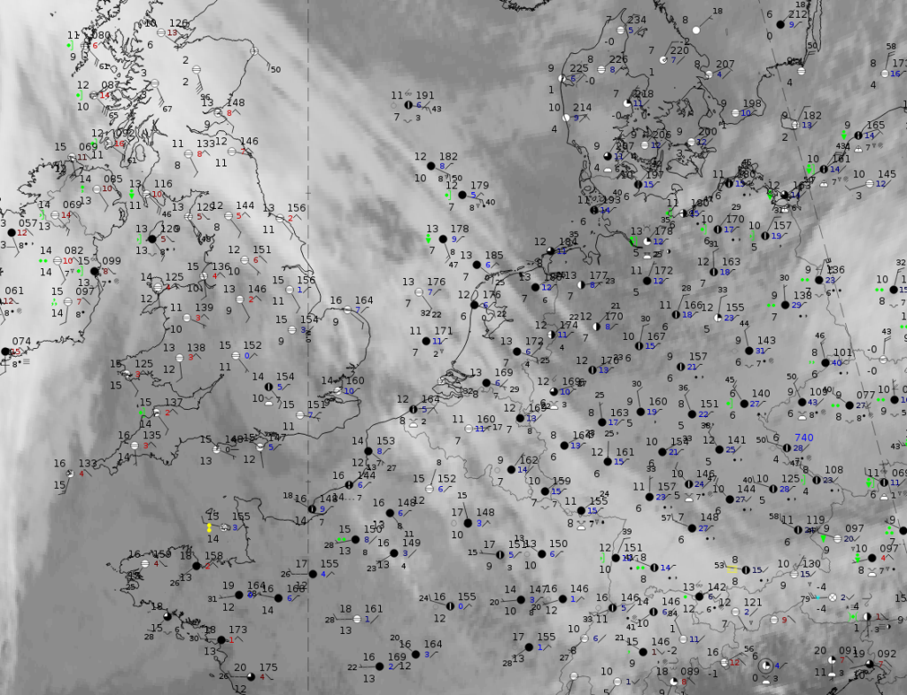
The following example represents the location "at the rear of a synoptic scale trough".
|
|

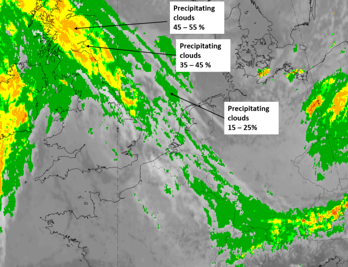
5 October 2019, 12UTC: IR + synoptic measurements (above) + probability of moderate rain (Precipitting clouds PC - NWCSAF).
Note: for a larger SYNOP image click this link.
The images show only very few shower and rain reports and the precipitation probability is generally very low, being higher only in the transition area between the warm front and the baroclinic boundary over Scotland. (link to legends)
|
|
|
|
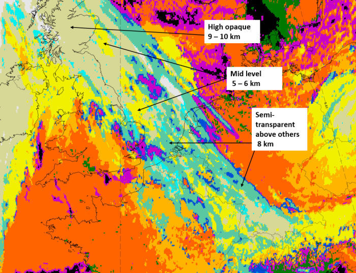
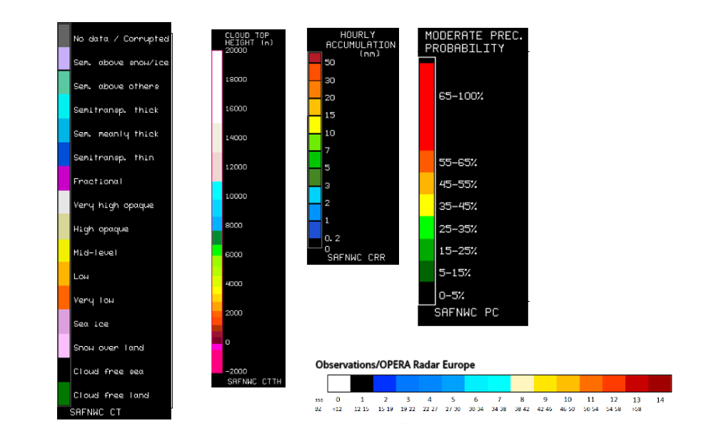
5 October 2019, 12 UTC, IR ; superimposed:
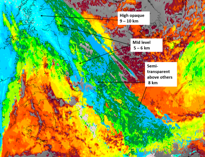
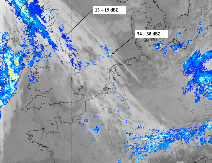
1st row: Cloud Type (CT NWCSAF) (above) + Cloud Top Height (CTTH - NWCSAF) (below); 2nd row: Convective Rainfall Rate (CRR NWCSAF) (above) + Radar intensities from Opera radar system (below).
For identifying values for Cloud type (CT), Cloud type height (CTTH), precipitating clouds (PC), and Opera radar for any pixel in the images look into the legends. (link)
References
General Meteorology and Basics
- CARLSON T. N. (1980): Airflow through mid-latitude cyclones and the comma cloud pattern; Mon. Wea. Rev., Vol. 108, p. 1498 - 1509
- GREEN J. S. A., LUDLAM F. H. and MCILVEEN J. F. R. (1966): Isentropic relative-flow analysis and the parcel theory; Quart. J. R. Meteor. Soc., Vol. 92, p. 210 - 219
- HARROLD T. W. (1973): Mechanisms influencing the distribution of precipitation within baroclinic disturbances; Quart. J. R. Meteor. Soc., Vol. 99, p. 232 - 251
- HERZEGH P. H. and HOBBS P. V. (1981): The mesoscale and microscale structure and organization of clouds and precipitation in mid-latitude cyclones. Part IV: Vertical air motions and microphysical structures of prefrontal surge clouds and cold frontal clouds; J. Atmos. Sci., Vol. 38, p. 1771 - 1784
- KURZ M. (1998): Synoptic Meteorology - 2nd complete revised edition, Deutscher Wetterdienst
General Satellite Meteorology
- BADER M. J., FORBES G. S., GRANT J. R., LILLEY R. B. E. and WATERS A. J. (1995): Images in weather forecasting - A practical guide for interpreting satellite and radar imagery; Cambridge University Press
Specific Satellite Meteorology
- BROWNING K. A. (1985): Conceptual models of precipitation systems; Quart. J. R. Meteor. Soc., Vol. 114, p. 293 - 319
- HOSKINS B. J. and HECKLEY W. A. (1981): Cold and warm fronts in baroclinic waves; Quart. J. R. Meteor. Soc., Vol. 107, p. 79 - 90