Table of Contents
Cloud Structure In Satellite Images
The best method for detecting Atmospheric Rivers (AR) over the oceans is to identify narrow stripes of high total column water vapor in the microwave spectral bands of polar-orbiting (LEO) satellite sensors. Satellite products showing the latest overpasses of LEO microwave sensors, such as the NDE blended Total Precipitable Water product, are the first choice when looking for ARs. Once ARs pass over land, their band-like structure rapidly dissolves due to surface friction and/or lifting.
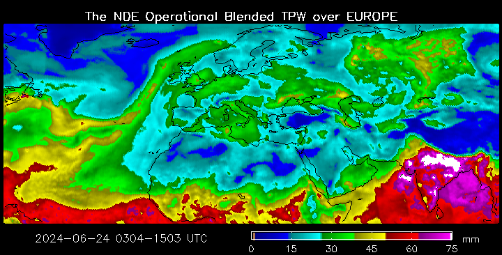
Figure 1: The NDE blended Total Precipitable Water (TPW) product is derived from polar-orbiting and geostationary satellite sensors including AMSU/MHS, SSMIS, ATMS and GPS Met. © NOAA NESDIS.
ARs are often accompanied by low clouds. For GEO satellites, ARs are best seen in visible imagery due to the higher contrast between low clouds and water compared to thermal imagery. Water vapor absorption channels from current geostationary satellites do not show these low-level moisture bands as the humidity is located at altitudes not covered by the SEVIRI instrument – typically below 700 hPa. Convective activity is rarely observed as the ARs are stably stratified.
|
|
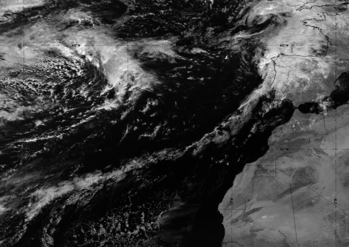
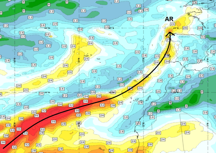
Figure 2: SEVIRI 0.8 µm VIS image from 2 April 2024 at 12:00 UTC. A narrow cloud band indicates the position of the AR over the Atlantic. Compare with the Total Column Water (TCW) product from ECMWF by using the slider.
|
|
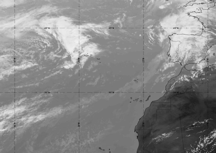
Figure 3: SEVIRI 10.8 µm IR image from 2 April 2024 at 12:00 UTC. A band of low clouds marks the AR located over the Atlantic. Compare with the TCW product from ECMWF by using the slider.
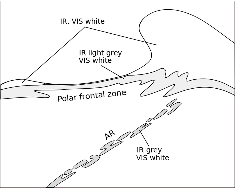
Figure 4: Schematic representing a frontal system and an AR in the grey shades used in VIS and IR.
The 24 hours Microphysics RGB is able to discern areas of higher and lower moisture in the lower troposphere using thermal infrared channels. High moisture values, which are found in ARs, are depicted in darker blue colors, while regions with less humidity tend toward a more pinkish color.
|
|
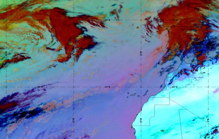

Figure 5: The 24 hour Microphysics RGB from 2 April 2024 at 12:00 UTC. Black lines indicate the low-level moisture boundaries. Use the slider to compare both images.
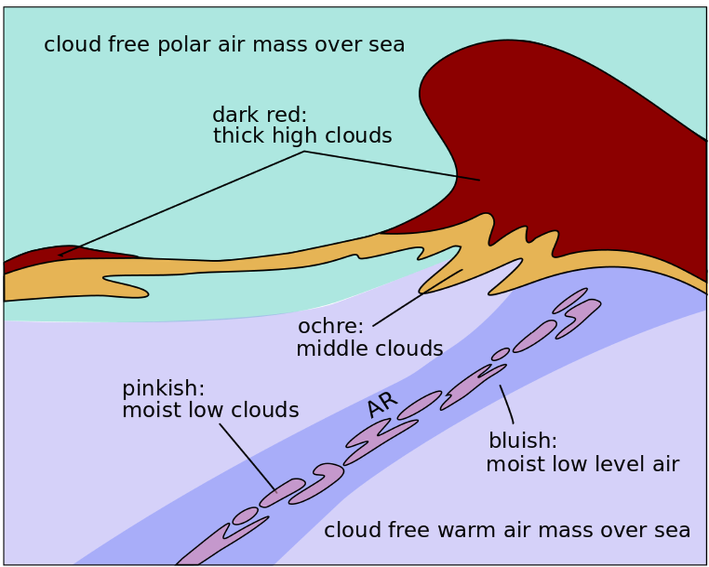
Figure 6: Schematic representing the color shades of an AR next to a frontal system in the 24 hour Microphysics RGB
Meteorological Physical Background
General Description
Atmospheric rivers (ARs) are low-level moisture bands emerging from a moist tropical air mass. They usually form over the seas and propagate polewards, later turning towards the east/west in the northern/southern hemisphere. ARs are frequent phenomena that are found in the region between the moist tropical air mass and the polar front. When they reach the polar front, they are often seen merging with the latter.
ARs are characterized by:
- A low-level moisture band (< 700 hPa).
- An initial water vapor content sourced from a moist tropical air mass or from a mid-latitude moisture source.
- A pronounced low-level jet along their way, which carries out the majority of the poleward moisture transport.
- Their location over the seas and rapid deterioration caused by friction and/or lifting upon making landfall.
- High amounts of precipitation during rapid lifting, such as when meeting mountains.
ARs should not be confused with the moisture bands found in the convergence zones of cold and warm fronts, nor with the Warm Conveyor Belt, which is a rising flow of warm and moist air ahead of a cold front.
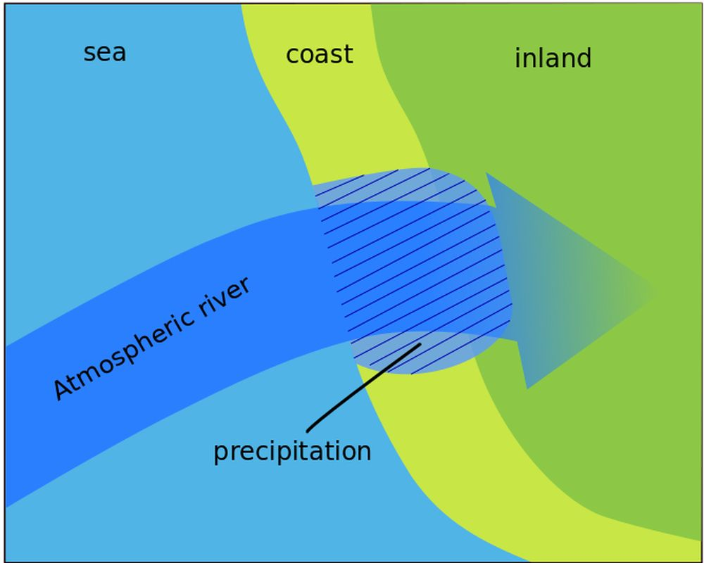
Figure 7: Schematic of an atmospheric river making landfall and being lifted by coastal orography.
Structure
- Atmospheric Rivers (ARs) are long and narrow bands of moisture in the lower troposphere that transport large amounts of water in liquid and gaseous form.
- ARs are defined as being at least 2000 km long and around 300 km wide on average with a total column water vapor (IWV) above 20 mm.
- Most of the humidity in ARs is found at levels below 700 hPa.
Location and origin of Atmospheric Rivers
ARs are located in the maritime tropical (mT) air mass, which consists of moist warm air. Influenced by pressure systems on their way north, they are typically found on the warm side of extratropical cyclones.
The initial water vapor supply in ARs stems from tropical moisture sources, from which it is transported outside the tropics over thousands of kilometers. Additional moisture is supplied on the way by evaporation from the sea surface, ensuring that the base of the AR always contains enough moisture. In addition, pre-frontal convergence helps maintain high total column water vapor.
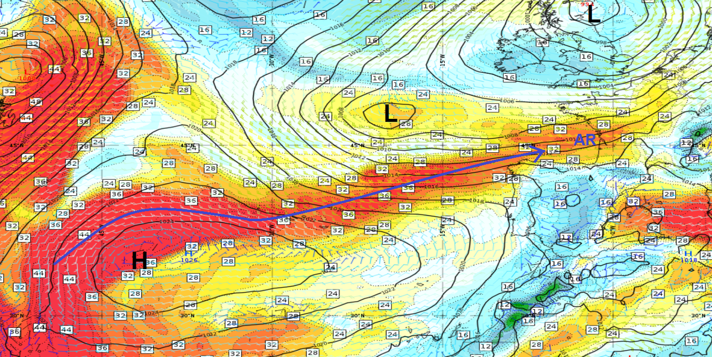
Figure 8: AR (blue arrow) shown in the Total Column Water parameter (ECMWF) on 16 June 2024 at 09:00 UTC. Mean Sea Level Pressure (black) and Wind barbs at 850 hPa.
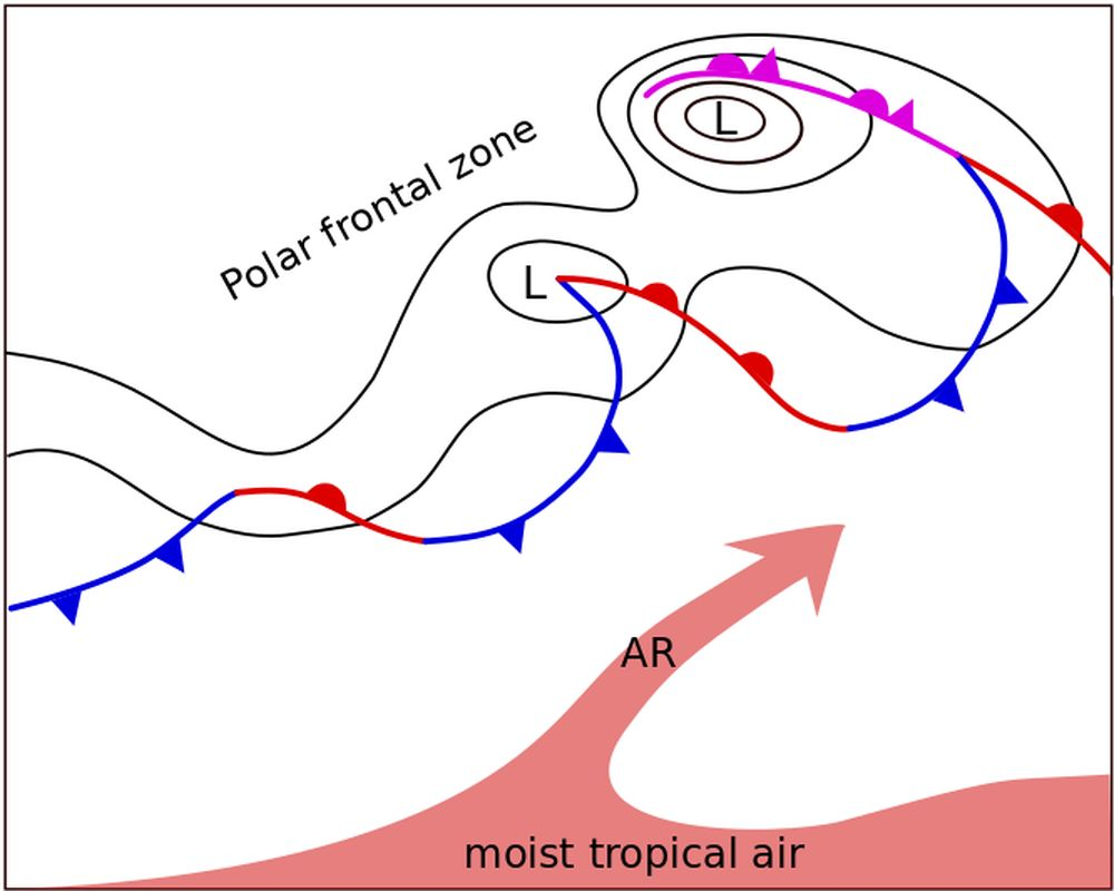
Figure 9: Schematic of the location of an AR compared
to the polar front.
Upon landfall, the river's typical elongated shape rapidly deteriorates and the amount of precipitable water decreases. ARs can cause precipitation and flooding, especially if the moist air is forced to ascend near the coast or in a mountainous region.
Evolution of Atmospheric Rivers: Merging and deformation
ARs are often observed converging with the polar front as they move north. When this happens, the moisture band of the AR becomes mixed with the moisture band of the polar front. Under these conditions, the AR is integrated into the pre-frontal moisture band and cannot be differentiated (see chapter IV on appearance in vertical cross sections).
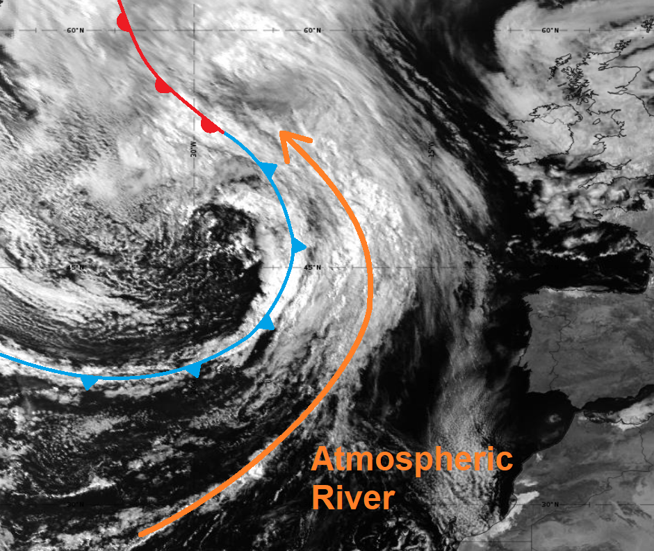
Figure 10: SEVIRI VIS 0.8 µm image from 24 May 2024 at 09:00 UTC.
AR merging with a cold front.
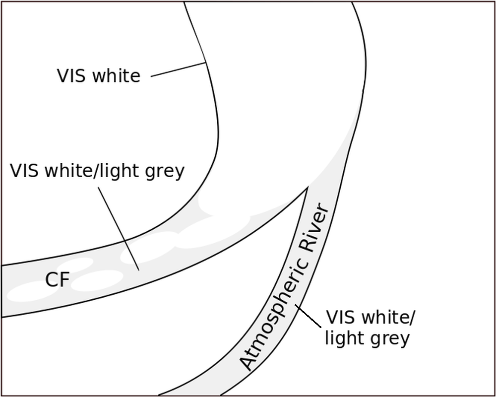
Figure 11: Schematic of an AR merging with a cold front.
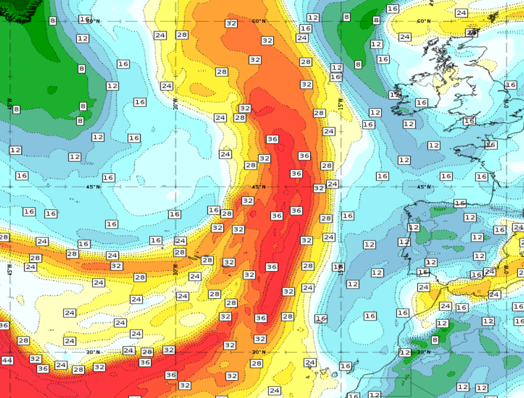
Figure 12: Total Column Water (TCW) from 24 May 2024 at 09:00 UTC.
Merging of the high moisture bands of the cold front and the AR.
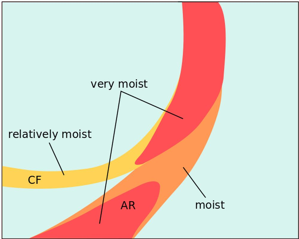
Figure 13: Schematic of the TCW amount in a merging process of an
AR with a clod front.
These narrow ribbons of low-level moisture often undergo transformations over time. When influenced by high and low pressure systems, these bands can be stretched, compressed or bent in various ways. Under these circumstances, ARs do not show a unidirectional wind field from source region to the very end of the AR. Wind direction can even become reversed when the AR is stretched or deformed by changing pressure gradients.
Figure 14: AR loop from 23 to 24 May 2024. Total Column Water (ECMWF) (top left), Airmass RGB (top right), relative humidity at 850 hPa (bottom left) and wind barbs at 850 hPa (bottom right) superimposed on the SEVIRI IR10.8 µm image.
Distinction from the Warm Conveyor belt
- ARs are not identical to the Warm Conveyor Belt (WCB), although they can be found in the same place. While a WCB rises continuously ahead of a cold front to eventually reach the upper troposphere, an AR remains at altitudes below 700 hPa. A WCB and an AR can be superimposed on each other.
- ARs are always accompanied by a low-level jet (LLJ). These strong near-surface winds induce an intense moisture transport from the tropics to mid-latitude regions.
- WCBs are relative streams that are defined with respect to a particular extratropical cyclone. In contrast, ARs are usually not connected to a single extratropical cyclone; instead, they remain in the warm sector of a succession of extratropical cyclones.
Key Parameters
The key parameters of an Atmospheric River (AR) refer are:
A. The position relative to fronts
B. The moisture content
C. The associated wind field
A. The position of Atmospheric Rivers relative to fronts
Equivalent Potential Temperature
- ARs occur in warm and moist air masses, typically in the warm sector of a frontal system but also in the warm air south of the polar front.
|
|
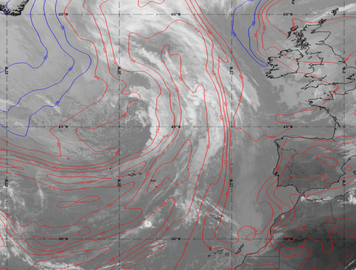
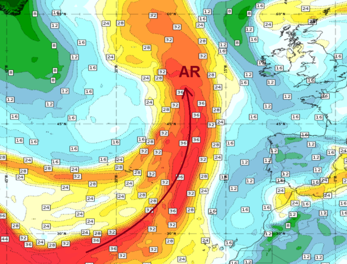
Figure 15: SEVIRI IR
10.8 µm image with Theta-e at 850 hPa and Total Column Water (ECMWF) from
24 May 2024 at 09:00 UTC.
Use the slider to
compare both images.
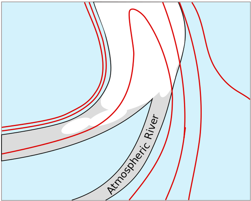
Figure 16: Schematic of the Equivalent Potential Temperature at 950 hPa in respect to the position of the AR.
Atmospheric Thickness 500 - 1000 hPa
- The ARs are located in the ridge of the atmospheric thickness parameter.
- When the AR converges with the polar front, they are found near the gradient zone of the thickness parameter – still on the warm side.
|
|
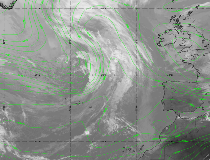
Figure 17: SEVIRI IR
10.8µm image with thickness 500-1000 hPa and Total Column Water (ECMWF)
from 24 May 2024 at 09:00 UTC.
Use the
slider to compare both images.
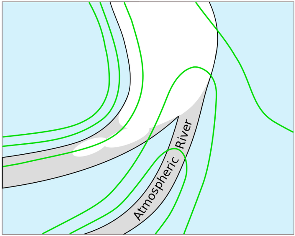
Figure 18: Schematic of the Atmospheric Thickness parameter (500-1000hPa) in respect to the position of the AR.
B. Moisture content in Atmospheric Rivers
Relative humidity and Total Column Water
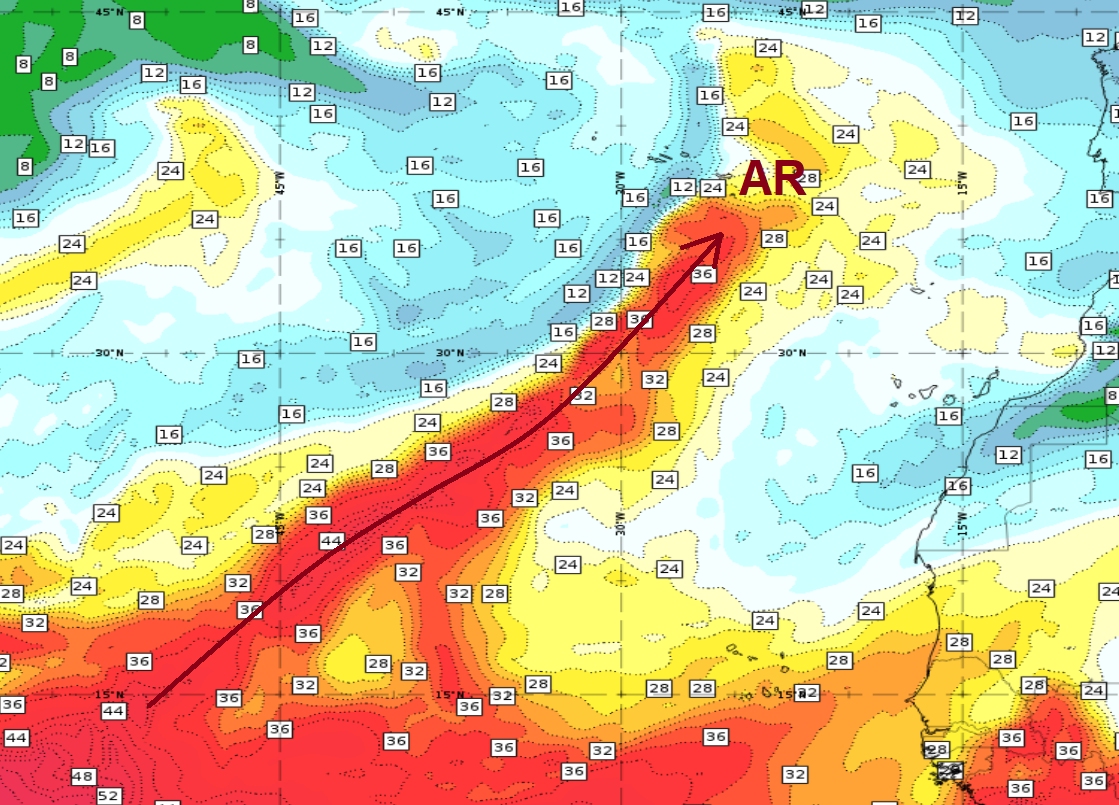
Figure 19: Total Column Water (ECMWF) on 1 April 2024 at 12:00 UTC.
- ARs are characterized by high relative humidity values in the lower troposphere, typically up to around 700 hPa and by total column water values of more than 20 mm.
- Their initial moisture supply comes from a maritime tropical air mass.
- The atmosphere above the AR (typically higher than 700 hPa) is dry.
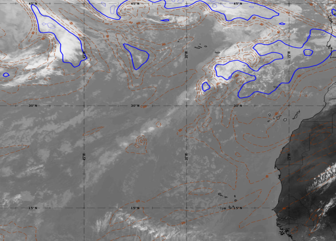


Figure 20: Relative humidity (ECMWF) at 500 (top), 700
(middle) and 850 hPa (bottom) superimposed on SEVIRI
IR10.8 µm image from 1 April 2024 at 12:00 UTC.
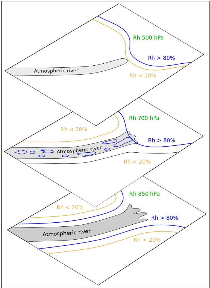
Figure 21: Schematic of relative humidity (Rh) at corresponding levels.
C. The wind field
- ARs are usually associated with stronger winds in the lower levels, the so-called low-level jets. The low-level wind field often shows a convergence along the humid belt.
|
|
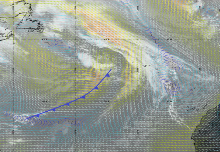
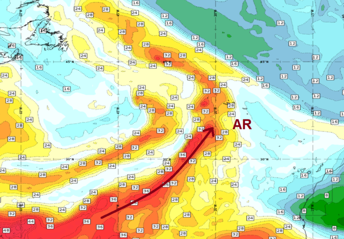
Figure 22: SEVIRI
IR 10.8 µm image with wind barbs at 950
hPa and Total Column Water (ECMWF) from 1 May 2024 at 18:00 UTC.
The
blue line indicates the cold front and brown arrow indicates the AR. Use the slider to
compare both images.
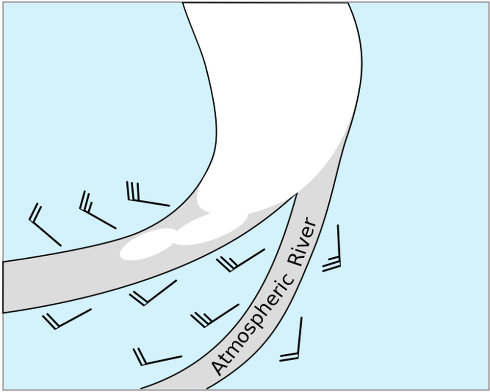
Figure 23: Schematic of surface wind convergence in the vicinity of an AR.
|
|
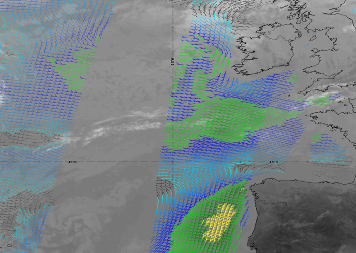
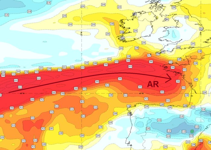
Figure 24: SEVIRI IR
10.8 µm image with ASCAT-B and ASCAT-C 10m
wind barbs and Total Column Water (ECMWF) from 22 July 2024 at 12:00 UTC.
The
brown arrow indicates the AR. Use the slider to
compare both images.
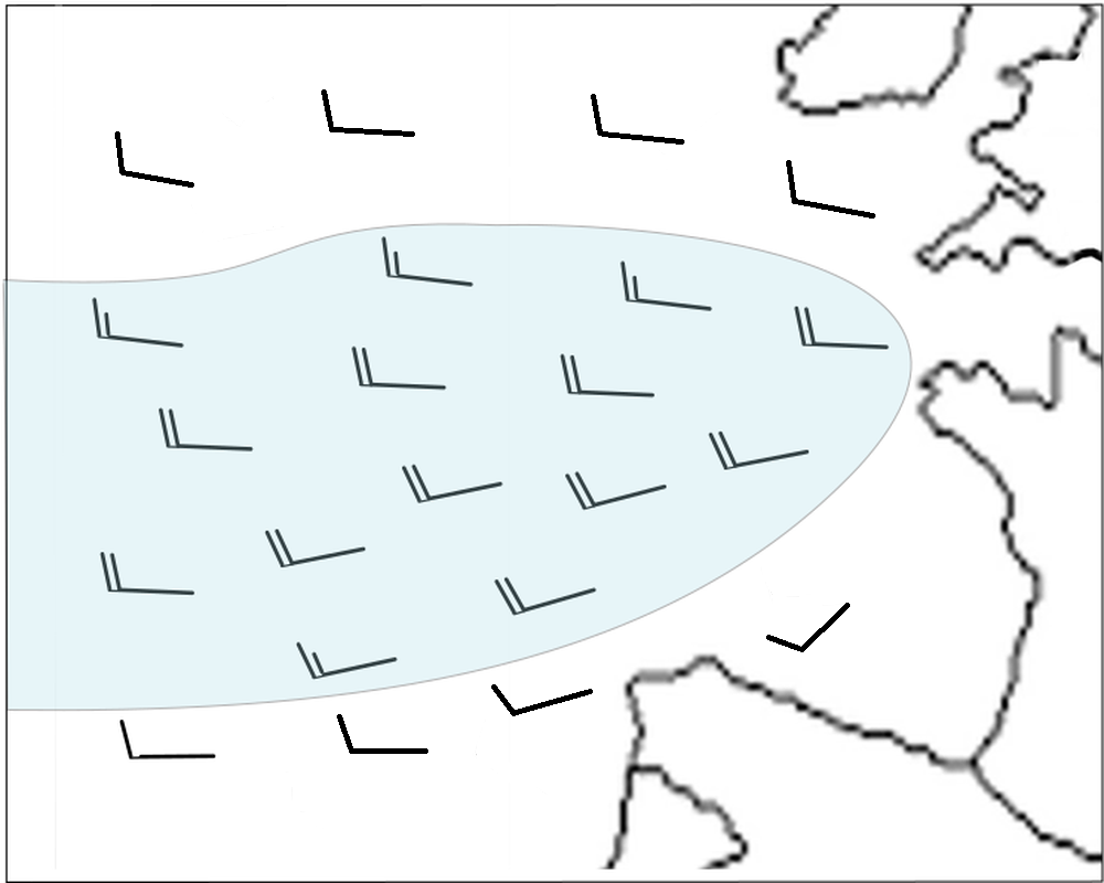
Figure 25: Schematic of 10m wind barbs over the ocean, inside (blue) and outside an AR.
Typical Appearance In Vertical Cross Sections
Wind, relative humidity and equivalent potential temperature show a characteristic pattern in an AR's vertical cross section.
- The relative humidity is high from the ground up to around 700 hPa, sometimes a little higher, when the AR is within the warm sector and separated from the polar front.
- The equivalent potential temperature (Theta-e) shows strong gradients on both sides and above the AR. These gradients are due to the AR's high water vapor content and not because of a temperature gradient.
- The wind speeds in an AR are typically higher than in its surroundings, and local maxima are often found in them.
Two different scenarios are discussed in more detail below:
- The moisture band of the AR is separated from the polar front.
- The AR undergoes a merging process with the moisture band of the polar front.
Case 1: The moisture band of the AR is separated from the polar front
- The vertical humidity profile shows a bulge of wet air up to 700 hPa with dry air above.
- The strong horizontal Theta-e gradients are due to the abundance of water vapor inside the AR.
|
|
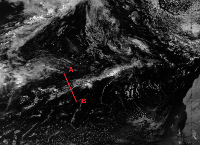
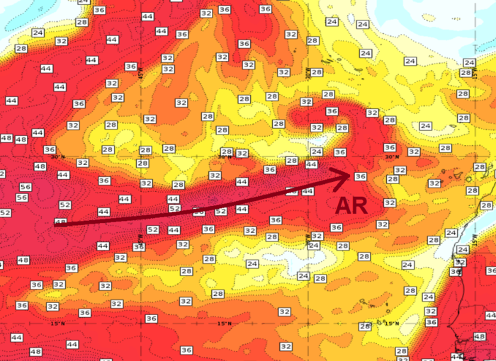
Figure 26: Total Column Water (ECMWF) and SEVIRI VIS 0.8 µm image from 9 June 2024 at 12:00 UTC. The red line idnicates the position of the vertical cross section and brown arrow indicates the AR. Use the slider to compare both images.
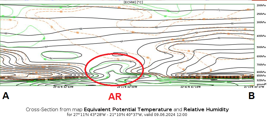
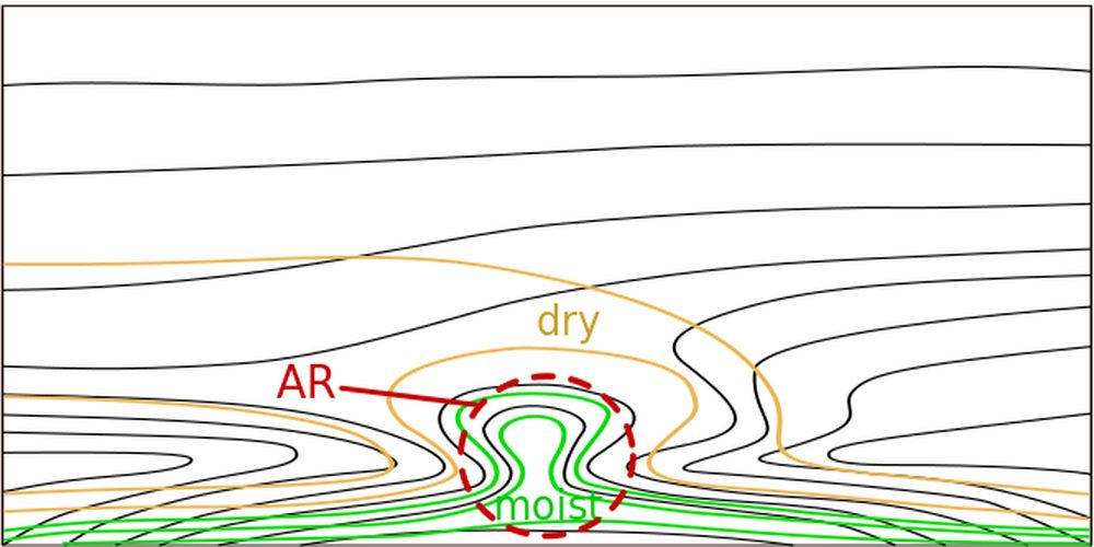
Figure 27: Vertical cross section through an isolated AR. Equivalent potential temperature [K] (black) and relative humidity [%] (green and brown) from 9 June 2024 at 12:00 UTC (left) and as a schematic (right).
- The vertical cross section below shows a local wind speed maximum in the area of the AR.
|
|
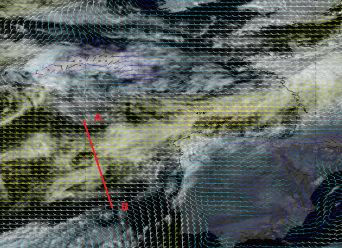
Figure 28: Total Column Water (ECMWF) and SEVIRI VIS 0.8 µm images with wind barbs at 950 hPa on 16 June 2024 at 12:00 UTC. The red line indicates the position of the vertical cross section and brown arrow indicates the AR. Use the slider to compare both images.
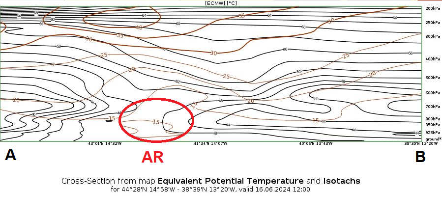
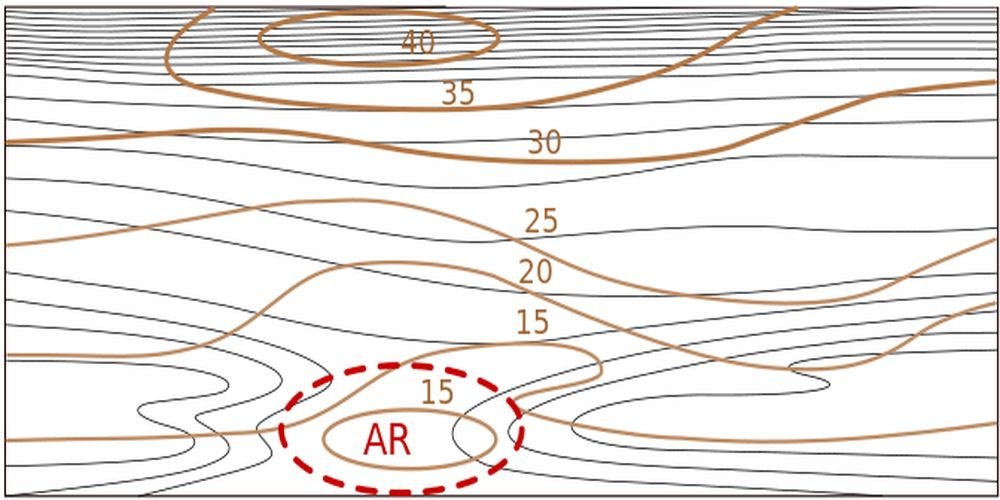
Figure 29: Vertical cross section through an isolated AR. Equivalent potential temperature [K] (black) and isotachs [m/s] (brown) from 16 June 2024 at 12:00 UTC (left) and as a schematic (right).
Case 2: The AR undergoes a merging process with the moisture band of the polar front
The case below shows an AR in the process of merging with the moisture band of a cold front. During this process, the AR continuously approaches the cold front from the warm side until both moisture bands merge. To illustrate this process, it is subdivided into two steps.
In the first step, the vertical cross section (i) shows the AR south of the merging point, still separated from the cold front. In the second step the VCS (ii) is positioned more to the north and shows the AR already merged with the pre-frontal moisture band of the katabatic cold front.
i. VCS located south of the merging point
- The low-level moisture field of the AR is separated from the moisture field of the cold front.
- The air above the AR is dry.
- A secondary low-level wind speed maximum can be observed as well.
|
|
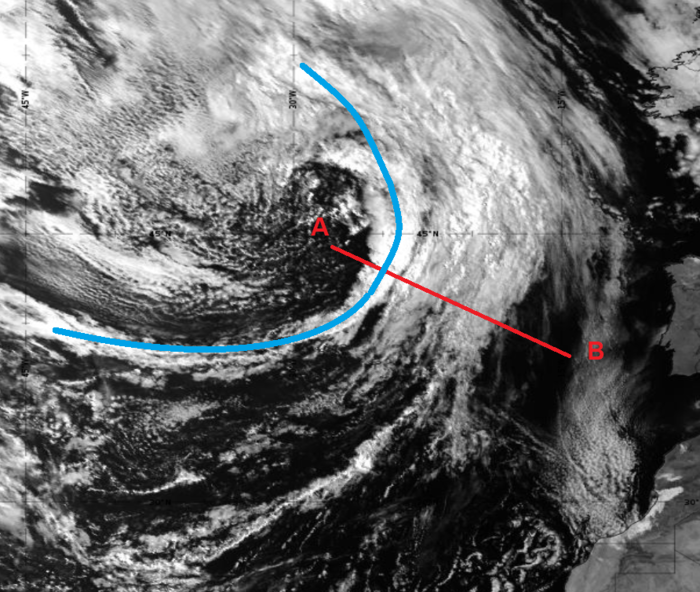
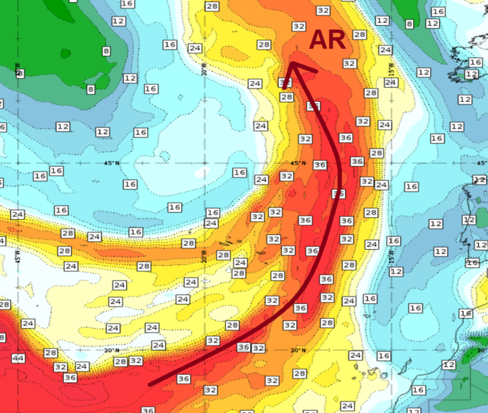
Figure 30: SEVIRI VIS 0.8 µm and Total Column Water (ECMWF) images from 24 May 2024 at 09:00 UTC. The red line is the vertical cross section, the blue line marks the cold front and the brown arrow indicates the AR. Use the slider to compare both images.
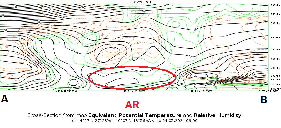
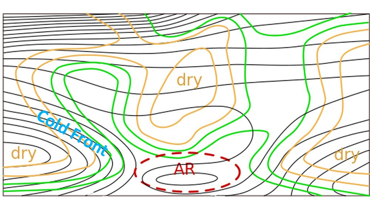
Figure 31: Vertical cross section through an isolated AR. Equivalent potential temperature [K] (black) and relative humidity [%] (green and brown) from 24 May 2024 at 09:00 UTC (left) and as a schematic (right).
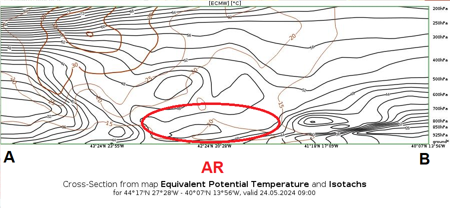
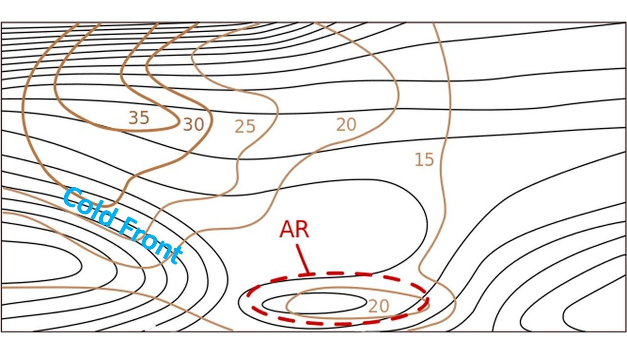
Figure 32: Vertical cross section through an isolated AR. Equivalent potential temperature [K] (black) and isotachs [m/s] (brown) from 24 May 2024 at 09:00 UTC (left) and as a schematic (right).
ii. VSC located north of the merging point
- After merging with the polar front, pre-frontal humidity reaches from the surface up to the vertical limit of the cold front.
- The low-level jet associated with the AR is still prominent.
|
|
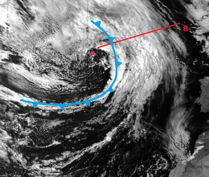
Figure 33: SEVIRI VIS 0.8 µm and Total Column Water (ECMWF) images from 24 May 2024 at 09:00 UTC. The red line is the vertical cross section, the blue line marks the cold front and the brown arrow indicates the AR. Use the slider to compare both images.
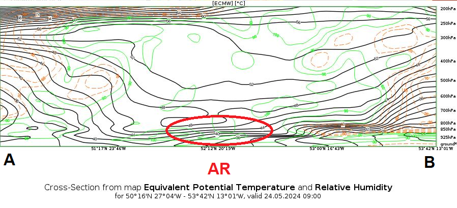
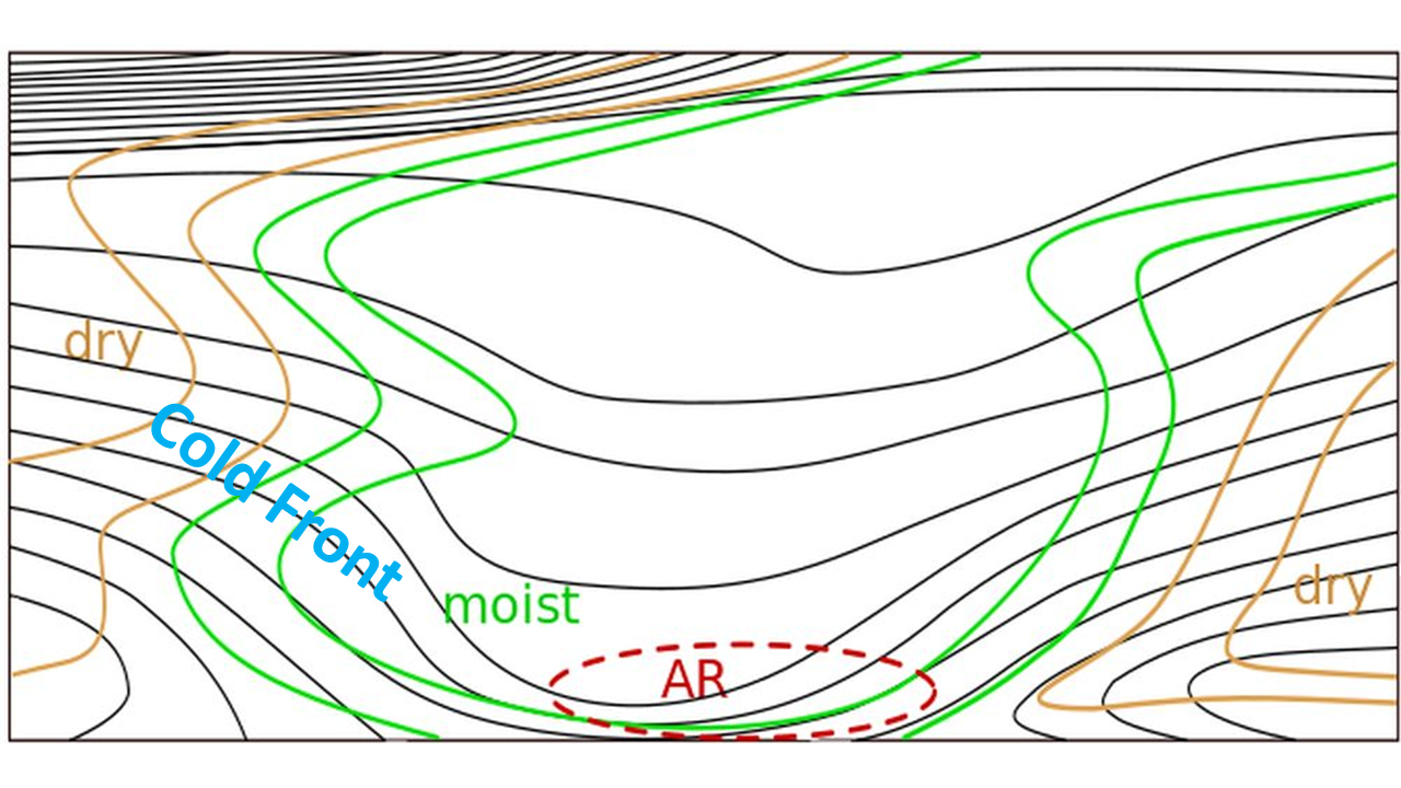
Figure 34: Vertical cross section through an isolated AR. Equivalent potential temperature [K] (black) and relative humidity [%] (green and brown) from 24 May 2024 at 09:00 UTC (left) and as a schematic (right).
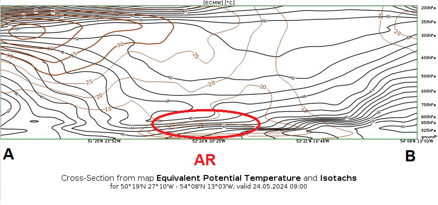
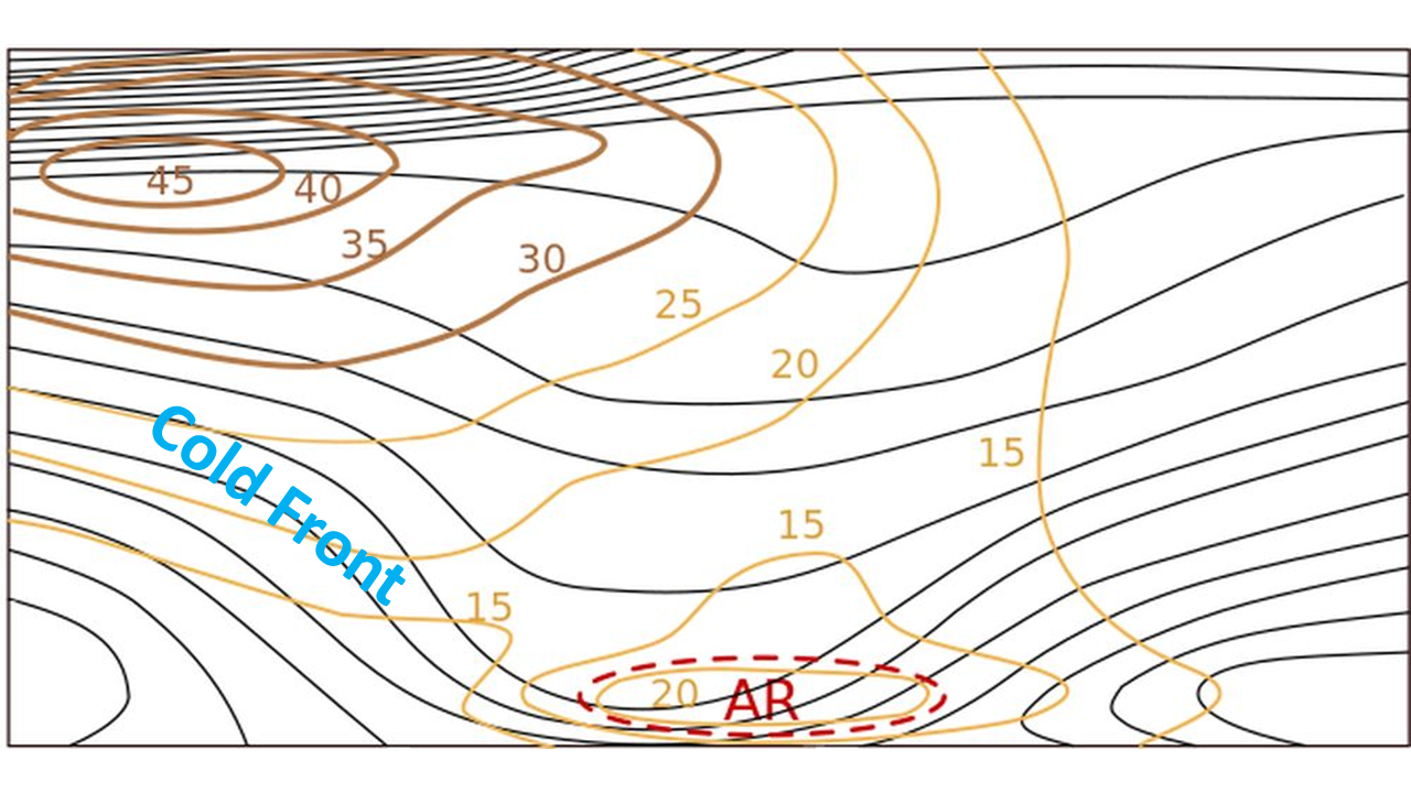
Figure 335: Vertical cross section through an isolated AR. Equivalent potential temperature [K] (black) and isotachs [m/s] (brown) from 24 May 2024 at 09:00 UTC (left) and as a schematic (right).
Weather Events
Atmospheric Rivers (AR) provide the majority of water vapor transport from the tropics towards the mid-latitudes and are associated with episodes of heavy and prolonged orographic precipitation over land. While there is little precipitation above water, when the AR hits the coast and moves inland it can release massive amounts of rainfall, especially when the stream of wet and moist air is lifted over a mountain chain. These extreme precipitation events can lead to flash flooding, mudslides, and catastrophic damage to life and property.
ARs are responsible for many of the largest winter floods in the mid-latitudes as well as for many annual daily precipitation maxima in Western Europe. They can also trigger precipitation as far inland as Germany and Poland.

Figure 36: SEVIRI VIS 0.8 µm image form 29 May 2024 at
12:00 UTC. Streamlines
at 1000 hPa indicate the
advection of moist saturated air within an AR.
Green
symbols indicate precipitation over France.

Figure 37: Schematic showing where precipitation occurs
after an AR makes landfall.
The low-level winds that accompany ARs are generally stronger over the sea than over land where they are weakened by friction processes.
There is general agreement that ARs occur in Europe more frequently during the cold season when extratropical cyclones are located further south. Additionally, ARs cause more precipitation in winter because of the higher meridional temperature gradient over Europe. The precipitation intensity also depends on the duration of the event, the amount of transported water vapor and the strength of the low-level jet.
Table 1: Table of meteorological parameters affected by ARs.
| Parameter | Description |
|---|---|
| Precipitation | High precipitation amounts over land in case of orographic lifting. High precipitation amounts over land when the AR is stationary over a longer period. |
| Humidity | High relative humidity (up to around 700 hPa) mixed with clouds. |
| Wind | Low-level jet over the ocean, wind speed reduced by friction over land. |
| Cloudiness | Overcast, low-level clouds. |
Precipitation products such as the Precipitating Clouds product from the Nowcasting SAF or the Blended SEVIRI/LEO Precipitation Product from EUMETSAT show high likelihood of rainfall as soon as the AR reaches land.

Figure 38: SEVIRI VIS 0.8 µm image and Precipitating Clouds product [%] prob.] of the NWCSAF from 29 May 2024 at 12:00 UTC.

Figure 39: SEVIRI VIS 0.6 µm image and Blended SEVIRI / LEO Precipitation Product from 29 May 2024 at 10:00 UTC.
References
General information about Atmospheric Rivers:
NOAA: What are atmospheric rivers?
NOAA Research: Atmospheric Rivers: What are they and how does NOAA study them?
National Weather Service: Atmospheric River Brings Historic Rainfall to the Bay Area
Wikipedia: Atmospheric Rivers
Les Rowntree: What is An Atmospheric River, and How Does One Affect California's Rainfall?, Bay Nature magazine
Total Precipitable Water Product (NOAA):
General information: NESDIS Blended Total Precipitable Water (TPW) Products
bTPW Product: Atlantic Region
Literature on atmospheric rivers:
Ramos,A. M., Trigo, R. M., Liberato, M. L. R., and Tomé R.: Daily Precipitation Extreme Events in the Iberian Peninsula and Its Association with Atmospheric Rivers, Journal of Hydrometeorology, Vol. 16, Issue 2, 2015.
Guan, B., Waliser, D. E., and Ralph, F. M.: An Intercomparison between Reanalysis and Dropsone Observations of the Total Water Vapor Transport in Individual Atmospheric Rivers, Journal of Hydrometeorology, Vol. 19, Issue 2, 2018.
David A Lavers, Richard P Allan, Gabriele Villarini, Benjamin Lloyd-Hughes, David J Brayshaw and Andrew J Wade: Future changes in atmospheric rivers and their implications for winter flooding in Britain, Environ. Res. Lett. 8, 2013.
Jason M. Cordeira, F. Martin Ralph, Andrew Martin, Natalie Gaggini, J. Ryan Spackman, Paul J. Neiman, Jonathan J. Rutz, and Roger Pierce: Forecasting Atmospheric Rivers during CalWater 2015, Bulletin of the American Met. Soc., March 2017.
David A. Lavers and Gabriele Villarini: The nexus between atmospheric rivers and extreme precipitation across Europe, Geophys. Res. Letters, Vol. 40, 2013, 3259-3264.
Pasquier, J. T., Pfahl, S., and Grams, C. M.: Modulation of Atmospheric River Occurrence and Associated Precipitation Extremes in the North Atlantic Region by European Weather Regimes, Geophys. Res. Letters, Vol. 46, 2018, 1014-1023.
O. Rössler, P. Froidevaux, U. Börst, R. Rickli, O. Martius, and R. Weingartner: Retrospective analysis of a nonforecasted rain-on-snow flood in the Alps - a metter of model limitations or unpredictable nature?, Hydrol. Earth Syst. Sci., 18, 2265-2285, 2014.
H. F. Dacre, P. A. Clark, O. Martinez-Alvarado , M. A. Stringer, and D. A. Lavers: How do atmospheric rivers form?, Bulletin of the Amer. Met. Soc., August 2015, 1243-1255.
Ralph, F. M., Coleman, T., Neiman, P. J., Zamora, R. J., and Dettinger, M. D.: Observed Impacts of Duration and Seasonality of Atmospheric-River Landfalls on Soil Moisture and Runoff in Coastal Northern California, Bulletin of the Amer. Met. Soc., Vol. 14, April 2013, 443-459
Paul Froidevaux, Olivia Martius: Exceptional integrated vapor transport toward orography: an important precursor to severe floods in Switzerland, Quart. J. Roy. Met. Soc., Vol. 142, Issue 698, July 2016, 1997-2012.
F. Martin Ralph, Jonathan J. Rutz, Jason M. Cordeira, Michael Dettinger, Michael Anderson, David Reynolds, Lawrence J. Schick, and Chris Smallcomb: A scale to characterize the strength and impacts of atmospheric rivers, Bulletin of the Amer. Met. Soc., Vol. 100, Issue 2, Feb. 2019, 269-289.
Mahlstein, I., Bhend, J., Spirig, Ch., and Martius, O.: Developingan Automated Medium-Range Flood Awareness System for Switzerland Based on Probabilistic Forecasts of Integrated Water Vapor Fluxes, Bulletin of the Amer. Met. Soc., Vol. 34, Dec. 2019, 1759-1776.
David A. Lavers, Richard P. Allan, Eric F. Wood, Gabriele Villarini, David J. Brayshaw, and Andrew J. Wade: Winter floods in Britain are connected to atmospheric rivers, Geophys. Res. Letters, Vol. 38, 2011.