Chapter IX: Meteorological Products based on WV imagery
Table of Contents
- Chapter IX: Meteorological Products based on WV imagery
- Introduction
- Atmospheric Motion Vectors (AMV)
- MPEF Divergence Product (DIV)
- Air Mass RGB
- Literature
Introduction
As mentioned before in chapters 2 and 5, MSG WV channels are useful for locating PV anomalies or jet streaks and for deducing the general moisture distribution in the middle and upper layers of the troposphere. As a consequence both WV channels (6.2 and 7.3 µm) are also used to generate meteorological products and RGB composites. This chapter will present some of these VW based meteorological products and RGB combinations.
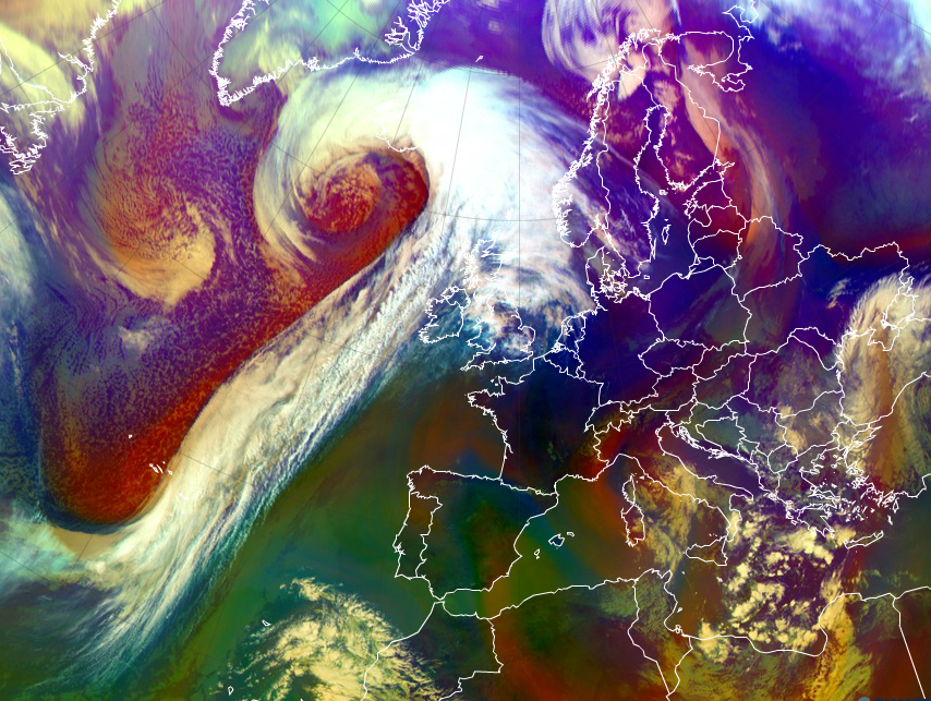
Figure 1: Airmass RGB from 8 March 2014, 12:00 UTC. This RGB composite image uses MSG WV channel 6.2 and 7.3 micrometer.
Atmospheric Motion Vectors (AMV)
The technique of tracking features in time sequences of satellite images for estimating atmospheric motions is used since the 1970s. Since then, the coverage and quality has notably improved mainly because of higher resolved image data and better algorithms but also because of the availability of WV channels.
The advantage of using WV images is that the AMVs can also be detected in cloud free areas and that their features are more conservative in time than features in IR or VIS images. An example for such a product is the NWC-SAF's High Resolution Wind Product (HRW). It produces a high quality field of AMV.
How are AMVs derived?
First, the feature to be traced or a candidate target has to be selected. Some preconditions have to be met when selecting a tracer cloud:
- The feature must be large compared to the resolution of the images
- The life-time of the feature has to be longer than the time interval of the tracking sequence
The second step is to track the target in a time series of images in order to determine its motion relative to a fixed location, and consequently, the wind vectors. This is done by using either the “Euclidean distance” method or the “cross correlation” method.
The derived vectors have to be assigned to a height. This is one of the trickiest and error-prone operations/steps in the processing chain. To deduce whether the sky is cloudy or cloud-free, one has to determine the brightness temperature of the selected target and calculate the temperatures for its base and top.
With the help of a NWP forecast model or – if no model is available – a climatological profile, the temperature values are converted to pressure values. Another algorithm then determines which of the two pressure levels best represents the displacement. In clear air conditions the AMV-height is assigned by using the pressure level derived from the WV brightness temperature.
There are certain post-processing procedures that follow the processing of the AMVs. They will only be given a cursory explanation here. The first post-processing step is to assign a quality index to every vector. This quality index is computed by checking wind direction, speed and vector consistency while comparing them with those of previous images.
Consistency with neighboring vectors and NWP model wind fields is then factored in. The quality index is a weighted average over these temporal, spatial and forecast tests.
Orographic flag calculation is another post-processing procedure. This is done only for AMVs over land, and its purpose is to detect and reject vectors that are affected by the ground (e.g. orographic clouds).
Applications
AMVs are the only observations that provide a good coverage of upper tropospheric wind data over oceans and high latitudes. The observation and analysis of weather phenomena occurring in data-sparse regions will therefore profit from this data source.
Possible applications are:
- Tropical cyclones: AMVs are useful in depicting upper-level features. The data can also be used for forecasts or analyses and case studies. This means AMVs can help in understanding and forecasting a cyclone’s formation, intensity and track.
- AMVs can be used for analyzing meteorological conditions, especially over oceanic regions
- AMVs can be processed for assimilation into NWP models
- AMVs can be used for reanalysis of past synoptic situations
Figure 2 shows an example of AMVs computed by the SAF-NWC. The different colours denote different atmospheric levels. Changes in wind velocity and direction can be deduced from this product.
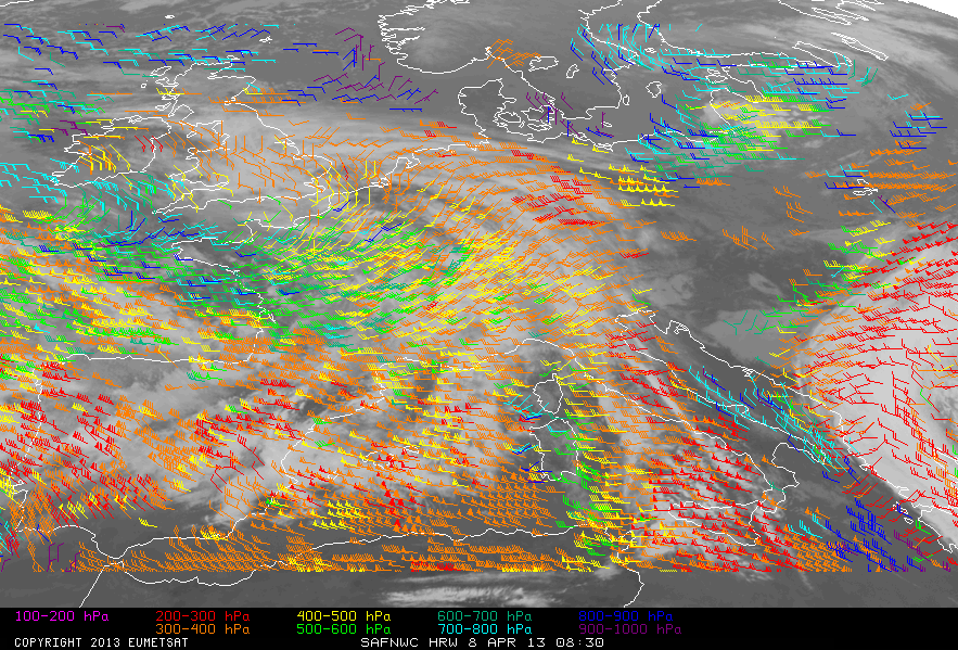
Figure 2: SAFNWC/MSG HRW AMVs for an area covering most of Europe and the Mediterranean: 08 April 2013 08:30 UTC (source: http://www.nwcsaf.org/)
Example: Hurricane Gordon
In September 2006 Hurricane “Gordon” first affected the Azores Islands as a hurricane and a few days later hit the north-western parts of the Iberian Peninsula as a tropical storm. In figure 3 the AMV analysis and the corresponding HRVIS satellite image of this date can be seen. The tropical storm is located in the south-western corner of the image connected to the southern end of a cold front. The surface low associated to Gordon can be detected quite clearly from the satellite image, but as the cyclone is completely embedded in the general flow of the cold front only a slight cyclonic deviation of the flow can be seen together with strong winds in lower layers.
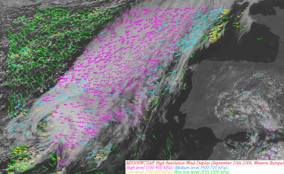
Figure 3: HRVIS image and AMV analysis of the tropical storm Gordon, 21 September 2006, 14:30 UTC.
Question
Find regions with upper level cyclonic and anticyclonic rotation.
- Solution: Click here to see these regions.
MPEF Divergence Product (DIV)
The MPEF Divergence product is calculated hourly by EUMETSAT and delivered to users via Eumetcast. The DIV product provides information about the upper-tropospheric flow, and more precisely about upper-level horizontal convergence and divergence.
This product is a special application of the WV AMVs. It uses AMVs from the WV 6.2 mm channel for deriving upper tropospheric divergence in order to forecast areas of deep moist convection. This is based on the fact that upper tropospheric divergence is the result of a strong updraft throughout the troposphere, which makes the area favorable for convection. The WV 6.2 µm channel is the best choice for this purpose, since it can track humidity features as well as clouds in the layer between 100 and 400 hPa.
Of note is that this product should be used in combination with instability parameters (for example GII) rather than by itself.
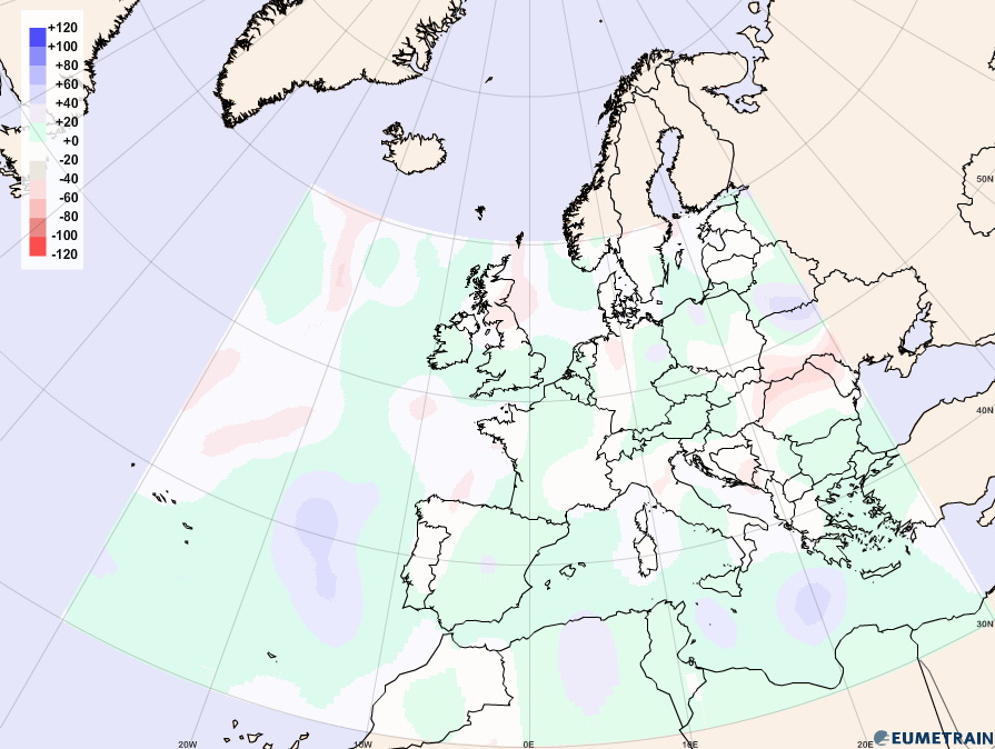
Figure 4a: MPEF DIV product, 13 June 2012, 12:00 UTC. Blue and green colors show divergence in upper tropospheric layers, red colors indicate convergence.
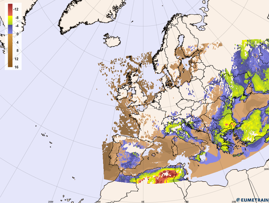
Figure 4b: Global Instability Index (GII), 13th June 2012, 12:00 UTC. The more negative the values are, the more unstable are the atmospheric conditions.
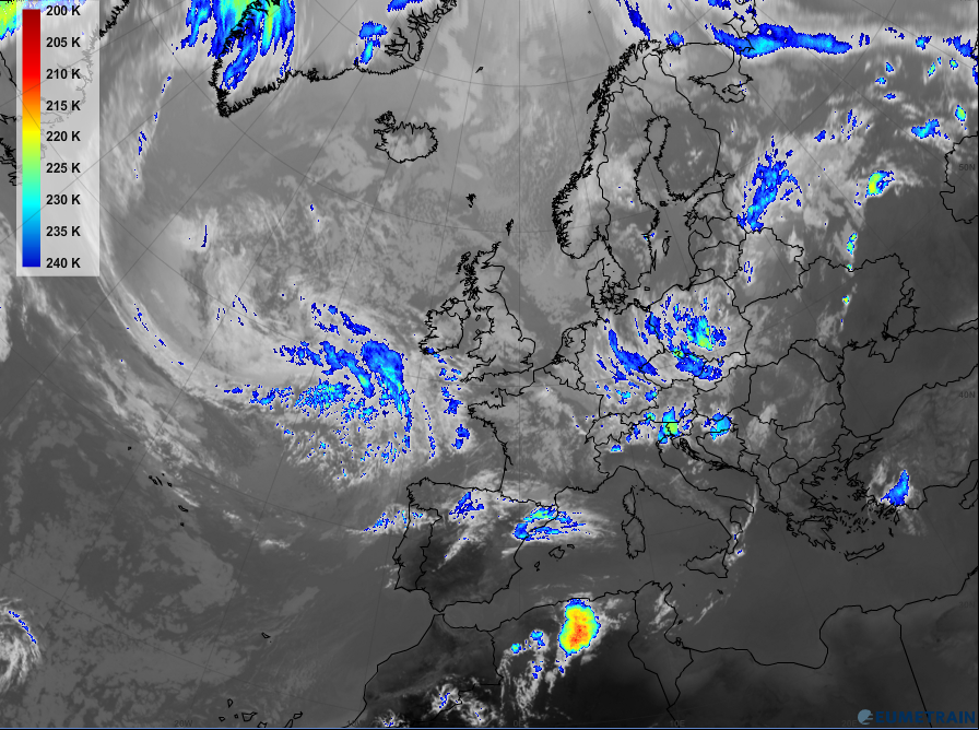
Figure 4c: Enhanced IR 10.8 µm image, June 13 2012, 18:00 UTC.
Figure 4a shows the MPEF DIV-field on 13 June 2012 at 12:00 UTC. Divergence in upper tropospheric layers (blue colours) can be detected west of the Iberian Peninsula, over North Africa and over the western Mediterranean Sea.
By comparing these regions with the GII fields (figure 4b), a distinct sign of instability can be seen over northern Africa. This is a region that forecasters should keep under observation in case there will be convective developments during the day.
Taking a look at the situation six hours later (figure 4c) a distinct convective cell has developed in this area.
Air Mass RGB
Just as every RGB composite, the Air Mass RGB combines several satellite channels in order to gain better information or highlight special features. As both water vapor channels (WV 6.2 µm and WV 7.3 µm) are included in this composite, the main applications are the detection of dynamic processes, such as rapid cyclogenesis, jet streams and PV anomalies.
Composition
The Air Mass RGB is composed as follows (figure 5):
- RED = Brightness temperature difference (WV6.2 – WV7.3)
- GREEN = Brightness temperature difference (IR9.7 – IR10.8)
- BLUE = Brightness temperature WV6.2
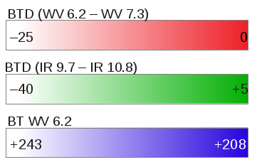
Figure 5: Composition and temperature range of the three colour beams of the Air Mass RGB.
The red beam reflects vertical water vapor distribution. A large proportion of red in the image is a sign of dry conditions at high levels.
The brightness temperature difference of the two IR channels on the green beam depicts an estimation of the tropopause height based on ozone concentration. A positive temperature difference is a sign of a high tropopause and tropical air mass.
The brightness temperature of the WV 6.2 µm channel on the blue beam shows the water vapour content in a layer between approximately 200 and 500 hPa. As the blue scale is inverted, moist upper levels and low brightness temperatures result in a large proportion of blue colour.
Applications
Air Mass RGBs can help detect areas of high PV advection (and therefore jet streaks and developing rapid cyclogenesis). The so-called stratospheric intrusions, where dry and ozone-rich air protrudes down into the troposphere, are shown in red to orange colors in the Air Mass RGB. They indicate zones of high PV advection.
The green component is small in these intrusions because the ozone concentration is large and the tropopause is low and warm. The IR9.7 channel's brightness temperature is therefore much lower than that of the IR10.8 channel. The WV6.2 brightness temperature is high, and therefore the blue component is also small.
Figure 6a and 6b show the WV 6.2 µm image and the Air Mass RGB from 19 October 2012 at 12:00 UTC. The dark stripes in figure 6a, showing dry areas in higher levels of the troposphere, can be clearly seen. The dark stripes of figure 6a appear red or deep orange in figure 6b. Note that the correspondence between the dark and red stripes only applies when the blue and green contributions are small, such as in the areas behind cold fronts.
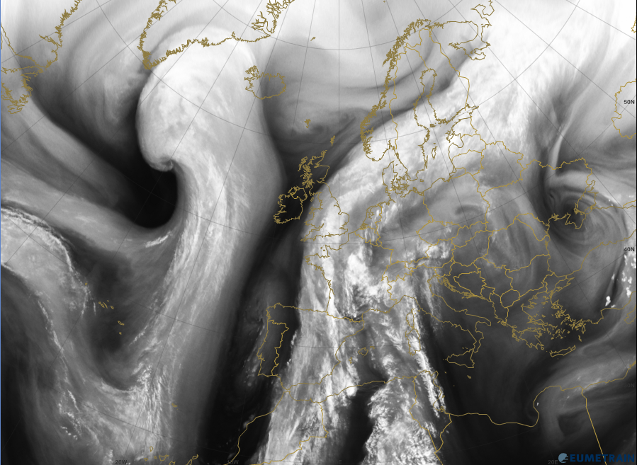
Figure 6a: WV 6.2 µm image, 19 October 2012, 12:00 UTC.
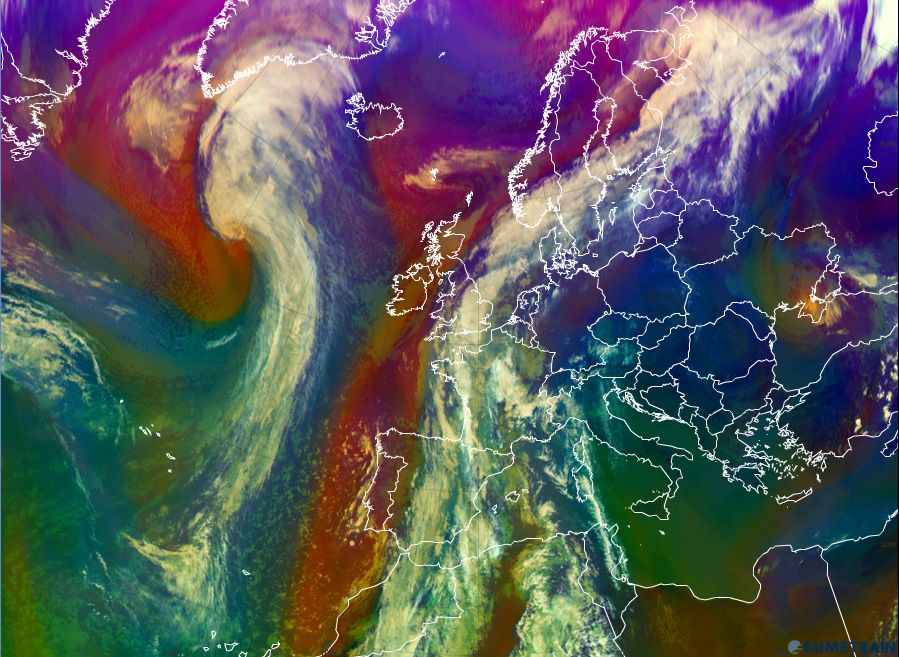
Figure 6b: Air Mass RGB, 19 October, 2012, 12:00 UTC.
When comparing the Air Mass RGB to the model PV=1.5 PVU surface height (figure 7), a clear correspondence can be observed between the red areas and PV anomalies. As mentioned earlier in chapter 2, dry stratospheric intrusions are a sign of potential vorticity advection to lower levels caused by conservation of PV. Therefore, when red or orange colors occur near fronts or occlusions in Air Mass RGBs, they can be an indication of rapid cyclogenesis or increasing destabilisation.
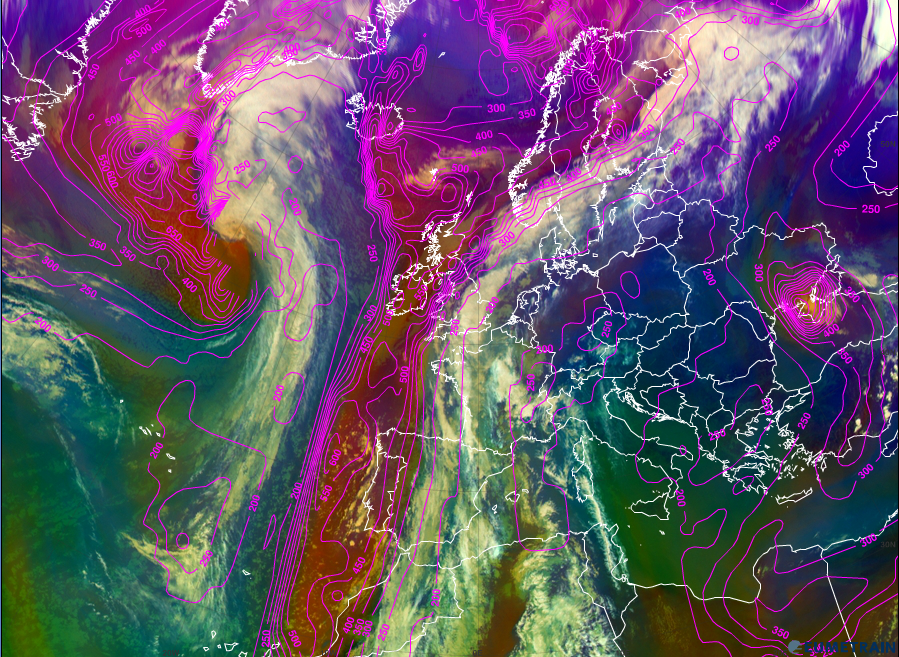
Figure 7: Air Mass RGB overlaid with 1.5 PVU surface height (pink), 19 October 2012, 12:00 UTC.
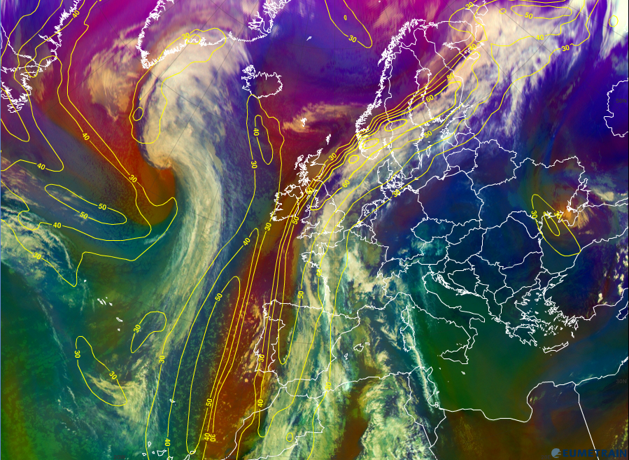
Figure 8: Air Mass RGB and ECMWF model field of the 300 hPa isotachs (yellow), 19 October 2012, 12:00 UTC.
The connection between dark stripes and the position of jet streaks was explained in previous chapters. As dark stripes connected to frontal rear sides correspond to orange or red stripes in the Air Mass RGB, this RGB can also be used for the location of jet axes. In figure 8 the Air Mass RGB is overlaid by the ECMWF model field of the 300 hPa isotachs. One can clearly see that the red stripes are on the cold side of the (model) jet axis.
As deformation zones can be detected with the help of a WV image loop (see chapter 6 for deformation zones), the same is also true for the Air Mass RGB loop. Figure 9 shows two deformation zones.
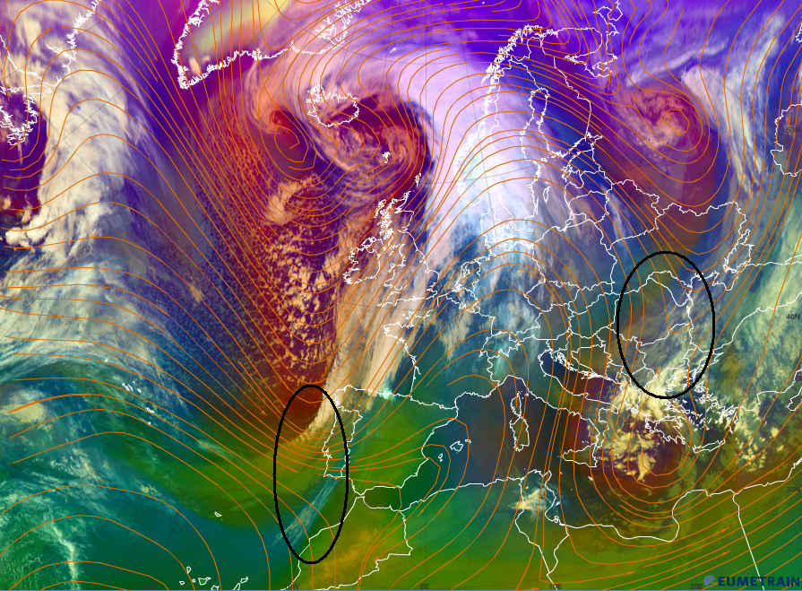
Figure 9: Air Mass RGB overlaid with the ECMWF model field of the 300 hPa streamlines, 29 December 2012, 06:00 UTC. The black circles mark the deformation zones.
Figure 10: Air Mass RGB loop from 03:00 UTC 09:00 UTC, 29 December 2012.
Notice:
| Red areas are not always showing areas of dry descending stratospheric air with high potential vorticity. |
Figure 11a shows a summertime Air Mass RGB image of the Middle East, where red colours are dominating the image. In this image the red to dark red colours indicate very high surface temperatures and low upper tropospheric humidity. A hint to discern dynamic tropopause anomalies from hot and dry areas: If the Air Mass RGB shows red colours because of high surface temperatures, those areas naturally only occur over land. For comparison one can look at the WV 6.2 µm image of the same date (figure 11b); no significant dark stripes can be seen there.
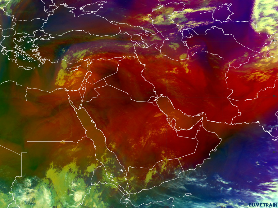
Figure 11a: Air Mass RGB over the Middle East, 22 June 2012, 06:00 UTC.
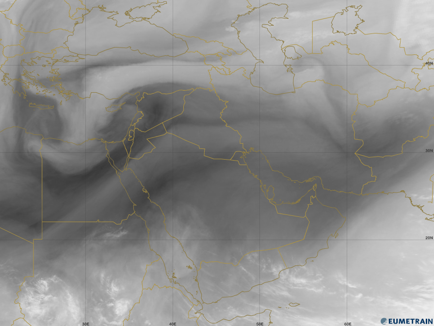
Figure 11b: WV 6.2 µm over the Middle East, 22 June 2012, 06:00 UTC.
Question
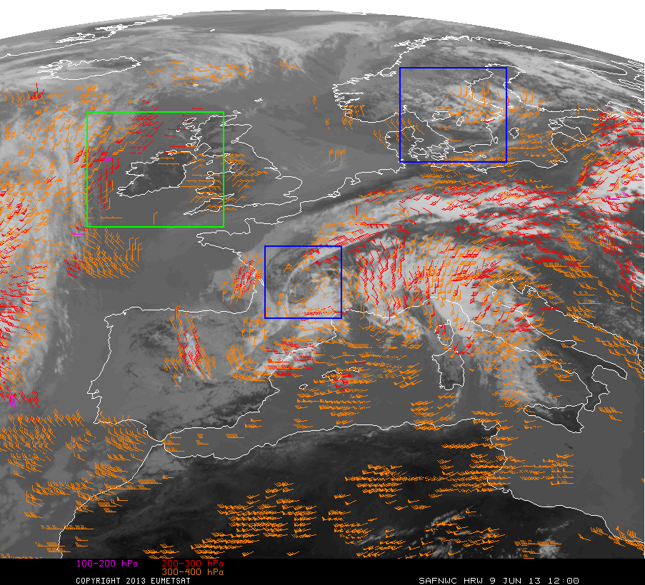
The image below shows an Air Mass RGB from 7 June 2013, 12:00 UTC. Try to find regions with descending dry stratospheric air.
Question
The image below shows an Air Mass RGB from 23 July 2012, 12:00 UTC. Try to find warm air masses.
Literature
Bader, M. J., Forbes, G. S., Grant, J. R., Lilley, R. B. E. and Waters, A. J.: Images in Weather Forecasting, Cambridge University Press, 1995.
Doswell, C. A.: The distinction between large-scale and meso-scale contribution to severe convection: A case study example. Weather and Forecasting, 2, 3ff, 1987.
Forsythe, Mary: ECMWF - Atmospheric Motion Vectors – past, present and future, ECMWF annual seminar 2007.
Georgiev, C.: Use of the MPEF Divergence product for diagnosing the environment of deep moist convection, Convection Week, 2011
Kuhl, C. T.: Studies in Forecasting Upper-Level Turbulence, Thesis, Naval Postgraduate School, Monterey, California, September 2006.
Liou, K. N.: An Introduction to Atmospheric Radiation, Second Edition, Academic Press, 2002.
Santurette, P. and Georgiev, C.: Weather Analysis and Forecasting, Applying Satellite Water Vapor Imagery and Potential Vorticity Analysis, Elsevier, 2005.
Shapiro, M. A.: Turbulent mixing within tropopause folds as a mechanism for the exchange of chemical constituents between the stratosphere and the troposphere, J. Atmos. Sci., 37, 994-1004, 1980.
Velden, C. S., Hayden, C. M., Nieman, S. J., Menzel, W. P., Wanzong, S., and Goerss, J. S.: Upper-Tropospheric Winds Derived from Geostationary Satellite Water Vapor Observations, B. Am. Meteorol. Soc., 78, 173195,1997
Wimmers, A. and Feltz, W.: Tropopause Folding Turbulence Product, Algorithm Theoretical Basis Document, May, 2010.