Introduction
According to the definition of CMs typical features have to be recognized in satellite images and numerical model fields. But which features are meant? In both images and isoline fields there are thousands of structures and features. Which ones are significant?
Example of identifying meteorologically significant features in both images and numerical parameters
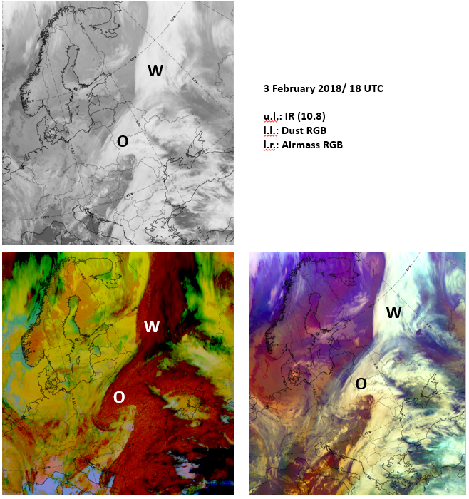 |
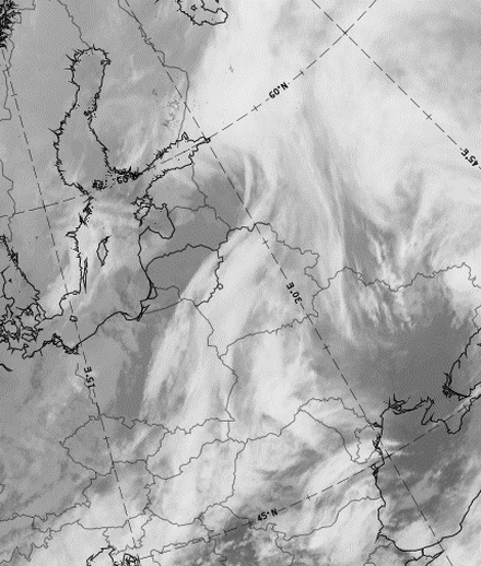
The case from 3 February 2018 at 18 UTC shows many cloud features in different scales: a synoptic scale cloud band extends from N to S; within this cloud band meso- to synoptic scale features like the substructures around W and O are very distinct; from the many small- to local scale cloud features cloud fibres can be recognized over France and the north coast of Turkey. Two cloud configurations will be discussed further:
The features just mentioned are typical for the CMs "Wave" and "Occlusion" as well as the physical process of cyclogenesis. |
Figure 1a-1c
The next step is investigating the typical features in numerical key parameters for these CMs within the region of the recognized cloud structures.
The key parameters for the CM "Wave" are taken from SatManu:
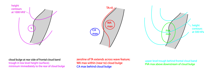
Figure 2
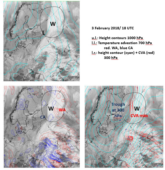 |
There is no distinct low in the low levels yet, but the WA and CA maxima within and at the rear side of the cloud bulge are well developed. The same is true for a distinct upper lever trough and a maximum of CVA situated in front of the trough over the cloud bulge. |
Figure 3a-3c
The cloud spiral around O can be diagnosed in the same way. An occlusion spiral is the end product of a cyclogenesis process and looks like a spiral cloud band together with cold and warm frontal cloud bands. It consists of thick clouds and gets a lumpy structure from convective clouds and embedded Cbs. These qualities are clearly visible in the 3 February 2018 case around the area O at 18 UTC.
The key parameters for the CM "Occlusion" are taken from SatManu:
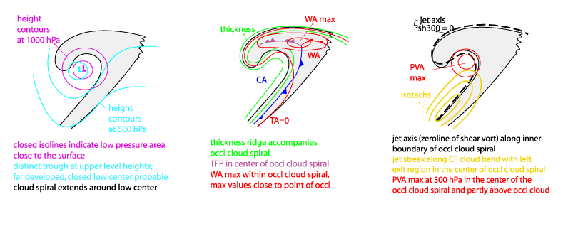
Figure 4
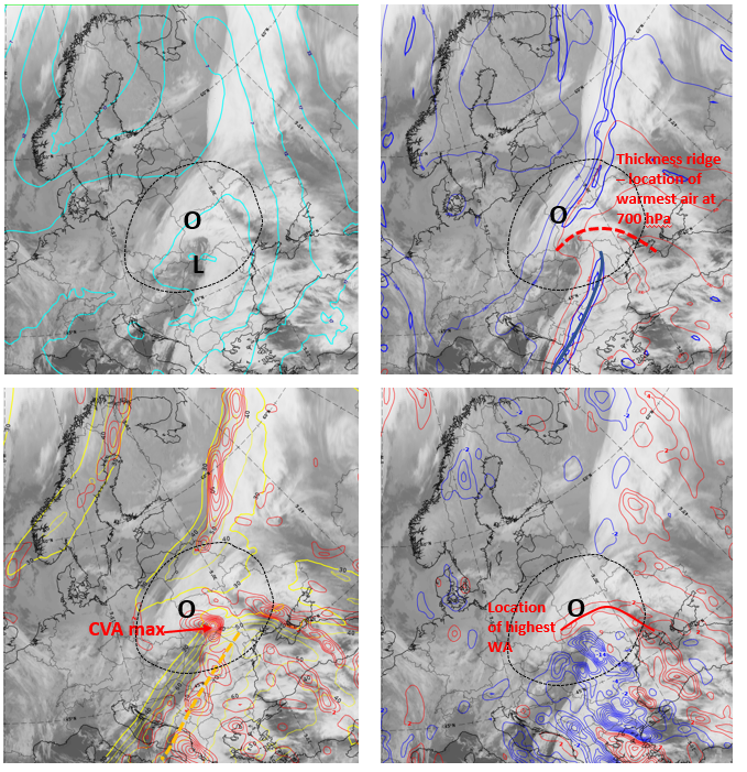 |
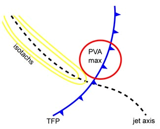
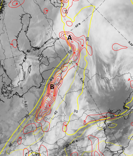
3 February 2018 at 18 UTC: Upper left: Height contours 1000 hPa Upper right: Thick blue: TFP. Thin solid lines (red, blue): theta-e 700 hPa. Dashed red: ridge line of theta-e 700. Lower left: Yellow: isotachs 300. Red: CVA 300 hPa. Dashed orange: jet axis 300 hPa. Lower right: Temperature advection at 700 hPa. Blue: CA. Red: WA. Thick red line: maximum of WA. |
Figure 5a-5d
Many of the features of the numerical key parameters are present: a low center in the low levels in the center of the spiral, a thickness ridge and an elongated maximum area of warm advection correspond to the cloud spiral. An intensive maximum of cyclonic vorticity advection (CVA) in the left exit region of the jet streak following the inner part of the occlusion cloud spiral is another common element.
For both CMs the relevant key parameters in the cloud area of the CM show the typical features (maxima, minima, ridges, ridge lines, etc.). This supports the initial choice of CM, settled on in the beginning by diagnosing the features found in satellite images, and the initial theory of what meteorological process might reasonably be expected to be causing them.
Starting from what is seen in the images and keeping to the area of those features is a crucial principle for the diagnosis of CMs described in SatManu.
Starting from a single feature of a typical key parameter - for instance a high level CVA maximum or the maximal change of a temperature gradient (thermal front parameter, TFP) - is not a useful approach to diagnosing an entire CM because doing so would ignore most of the parameter fields.
This can also be seen in the example treated previously; there are pronounced maxima of CVA, CA and WA in the region from eastern Balkan Peninsula to the Black Sea and Turkey, which is to the east and southeast of the occlusion cloud spiral (O) under consideration. Consequently, we can focus elsewhere and pose such question as: why are the most pronounced key parameter features outside the CM and not inside? Why are these strongest values not accompanied by cloud configurations typical of a CM?
The next paragraphs will answer and explain these issues.
Numerical parameters that contribute to upward motion like CVA maxima need not necessarily be related to cloudiness. One easy explanation for this is missing humidity. But even if cloudiness has formed as result of upward motion, the physical-meteorological processes suggesting a particular CM may be absent, or there might be another process going on. The CVA maximum in the center of the occlusion band O is clearly connected to the jet streak and the upper level trough at the rear of a frontal system; the CVA maximum over the eastern Black Sea and spreading into Turkey is in front of a cold front within warm advection, and therefore appears in a completely different physical-meteorological background. In diagnosing CMs one has to discern the meteorologically significant from less important features - filtering significant signals from noise.
This is not always easy and has to be learned. Three different situations are presented to demonstrate this.
Numerical key parameters show distinct features typical of specific CMs but are not accompanied by cloudiness
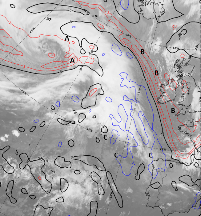
In the next example the thick blue lines show high values of the TFP. There are several lines, some of which are indicated by letters.
As demonstrated before, a basic step in using SatManu to diagnose CMs is to start from the cloud configurations and features in satellite images.
By following this advice, only the long north-south oriented TFP line A-A-A would be allocated to a frontal cloud system. But then, why are there other areas with high values of TFP? What do they signify?
Here is an example from 1 January 2018 at 12UTC:
 |
|
Figure 6a-6b
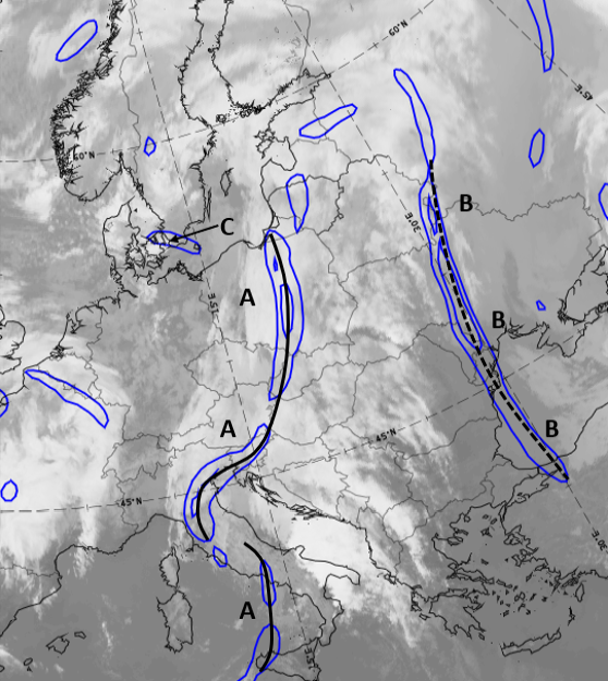
Thick blue: lines of high change of temperature gradient. Black: maximum line of change of temperature gradient.
Thin blue, red: theta-e 700 hPa.
Areas under discussion: A-A-A, B-B-B, C (south Sweden).
The thick blue lines are areas of high TFP values (maximal change of temperature gradient). In the example above the areas of interest are A-A-A, B-B-B and C, all of which show high TFP values. However, all of them characterize different physical-meteorological situations:
A-A-A:
- The TFP indicates the leading side of a zone of high theta-e gradients and is accompanied by cloud bands and spirals. The CM's cold front, warm front and occlusion can be assumed to be there.
B-B-B:
- In this region the dashed black line is located where there is a maximal change in the temperature gradient. However, there is no frontal cloudiness and therefore no frontal CM; it merely indicates the western side of a thickness trough. If additional meteorological processes occur there, a CM like "Air mass boundary" could develop.
C:
- Is already on a scale not appropriate for a frontal CM. Mathematically C does represent a maximal change of temperature gradient in the area but it has no physical-meteorological significance.
Maxima of numerical parameters contributing to upward motion in different meteorological surroundings
Maxima of CVA (cyclonic vorticity advection) contribute to upward motion and are therefore key parameters in several CMs. CVA maxima can be found in front of upper level troughs and/or in the left exit region of jet streaks. Still, not every CVA maximum is indicative of a CM described in SatManu.
Again, the demonstration uses a case from 1 January 2018 at 12 UTC.

Figure 7
Three areas of CVA maxima will be investigated in detail:
A:
- These very intensive maxima appear at the rear side of a cold front and occlusion cloud band and are therefore suggestive of CMs like "Front intensification by jet crossing" and/or "Rapid cyclogenesis" with an intensification in the left exit region. This has to be confirmed by considering the other key parameters of these CMs.
B:
- In this band-like CVA area there are intensive maxima but they are not accompanied by cloudiness; from the band-like orientation some connection to jet streaks can be supposed.
C:
- These centers of CVA are also not accompanied by cloudiness and their location to the south of frontal cloud bands does not recall any CM of SatManu.
But why do these maxima occur there, and what meteorological significance do they have?
 |
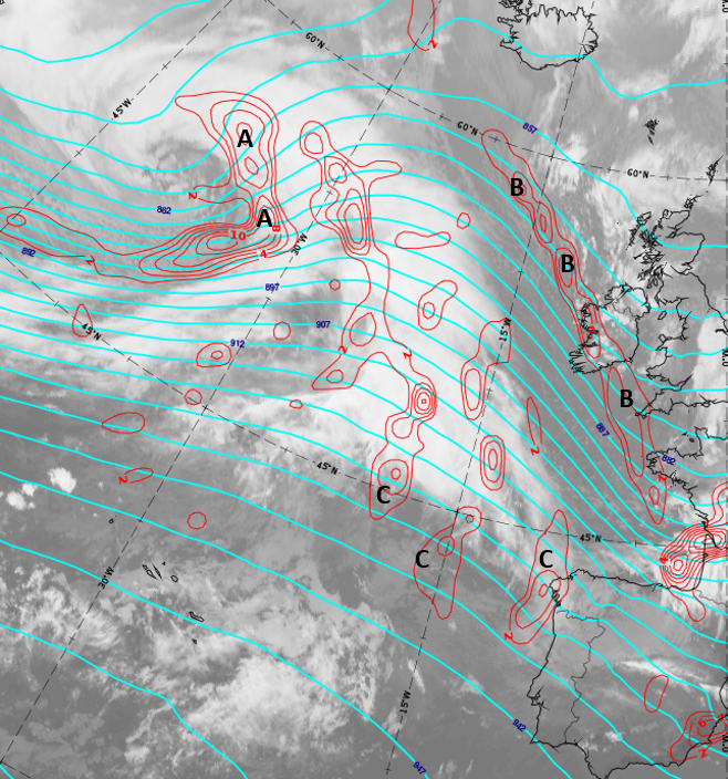 |
Figure 8a-8b
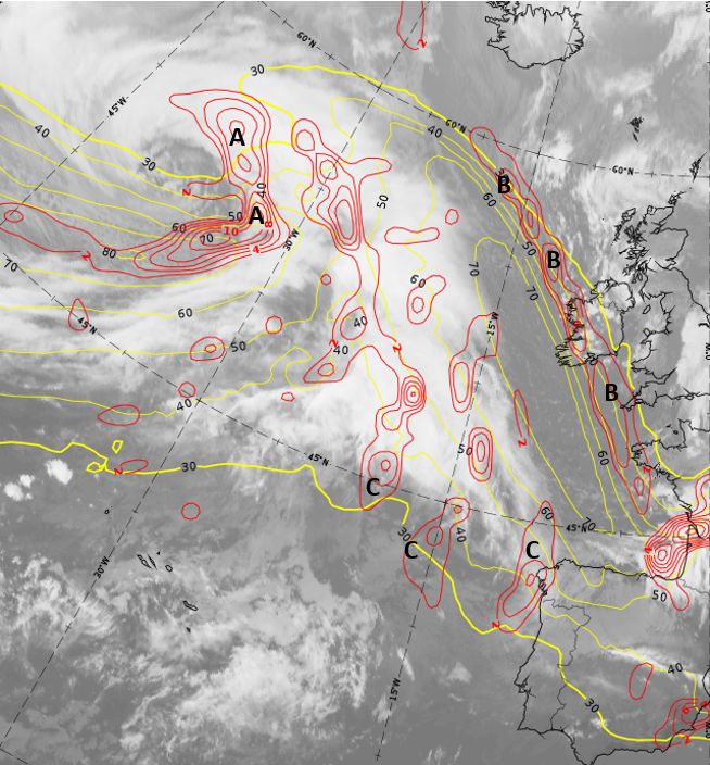
Red: CVA 300 hpa. Yellow: isotachs 300 hPa. Cyan: height contours 300 hPa.
A:
- The CVA maxima are in front of an upper level trough (high cyclonic curvature vorticity) as well as within a jet streak's left exit region (high cyclonic shear vorticity). The CMs mentioned above are supported by these key parameters and should be referenced for confirmation.
B:
- The CVA maxima are not in front of a height trough but on the cyclonic side of the jet streak. The relation to the jet streak can only be seen in the parallel orientation of the band of CVA maxima.
C:
- These CVA maxima do not have any relation to a height trough or a jet streak.
 |
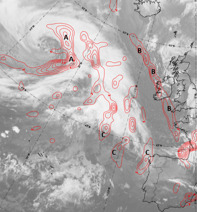 |
Figure 9a-9b
Left: relative vorticity 300 hPa.
Black: zero line. Red: cyclonic vorticity. Blue: anticyclonic vorticity.
Right: maxima of CVA 300 hPa.
A:
- The CVA maxima are on the leading side of maxima of relative vorticity, indicating areas where cyclonicity will increase. This is indeed the case for both frontal intensification by jet crossing as well as the left exit region of a crossing jet streak.
B:
- This band of CVA maxima running from northwest to southeast is in front of an elongated maximum of relative vorticity and, as it follows the cyclonic side of the NW-SE oriented jet streak, it represents cyclonic shear vorticity. The CVA maxima therefore indicate the eastward movement of the synoptic scale system.
C:
- These CVA maxima are at the rear side of anticyclonic vorticity maxima and indicate areas where anticyclonicity is decreasing. They are accounted for by mathematical models but in this position - south of a warm sector - do not have any meteorological importance as far as SatManu's CMs are concerned.
Influence of Numerical Model Resolution in Computation of Key Parameter Maxima in Different Scales
With better resolution of numerical models, more small-scale features are computed and they can sometimes have very intensive values. With a bigger grid distance of the model those small-scale features are mathematically filtered. Smaller grid distances allow recognition of smaller scale CMs but can also complicate the situation.
A very prominent example of this are derived numerical parameters like cyclonic vorticity advection. According to the omega equation CVA gives a positive input to upward motion (link). This is applied in the four quadrant model of jet streaks (link) where a CVA maximum can be found in the left exit region (an idealized case of this is called a straight jet streak). This is the explanation given by the CM "Front Intensification by Jet Crossing".
This is demonstrated in the following example from SatManu:
 |
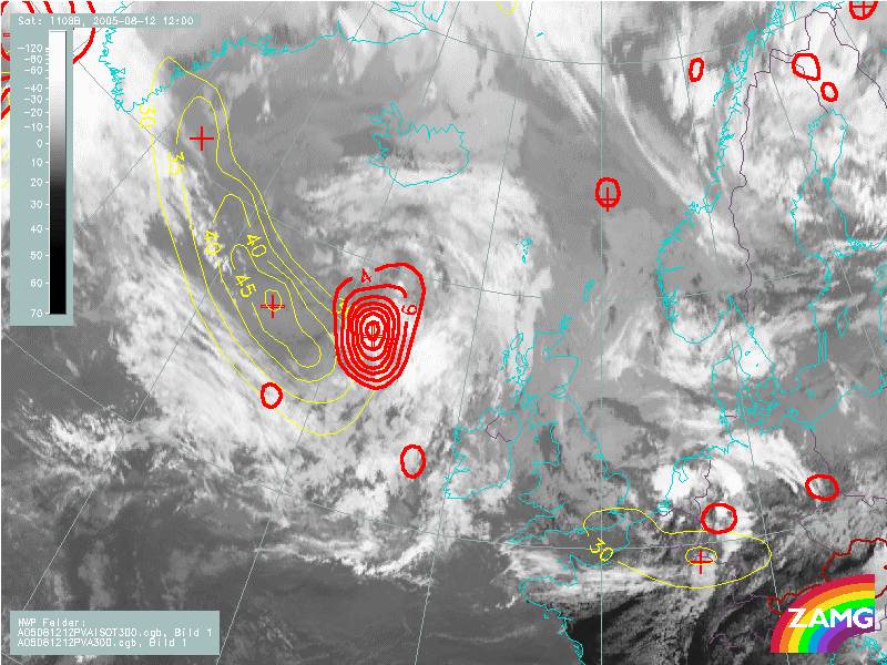 |
Figure 10a-10b
This very distinct CVA maximum in the left exit region of a nearly straight jet streak coincides with intensified cloudiness. This is a case from 12 August 2005 at 12 UTC where the numerical model had a much coarser grid resolution than several years later. A case from 2 February 2018 at 18 UTC is used for comparison. With a much smaller numerical model resolution many small-scale features are no longer filtered and might even appear more intensive than the features under consideration.
 |
 |
 |
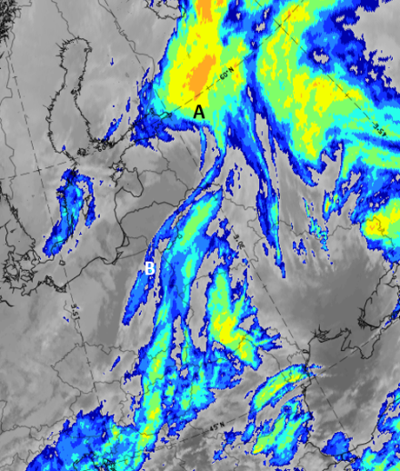 |
Figure 11a-11d
B is an elongated band of CVA maxima along the jet axis and shows even higher values than the CVA maximum A in the left exit region. Why does the CM refer to that smaller one and "ignore" the region with even more intensive maxima?
One reason is that the start of the diagnosis of a CM should be from the typical cloud configuration seen in satellite imagery. Around A a cloud spiral in a beginning occlusion stage with thick cloud and very cold cloud tops suggests occlusion cloud band as the CM. Around B a bulge at the rear side of the front cloud band could suggest the CM of a wave with a very sharp cloud edge built by a fibre with less cold tops.
From the location of the CVA maxima A and B, different physical processes can be identified in their development.
The vorticity maximum around A is on the cyclonic side of the jet streak's left exit region and accompanied by thick and very high cloud within a cloud spiral.
The elongated band of maxima B is in the center of the jet streak and consequently mirrors the very high vorticity gradients in the jet streak core (from cyclonic to anticyclonic values), which are mostly caused by the system's strong movement. The accompanying cloud fibre is also close to and parallel to the jet axis. A numerical model with a bigger grid distance would have filtered these small-scale features, while a smaller grid distance does not.
This can be confirmed easily by viewing the vertical cross sections:
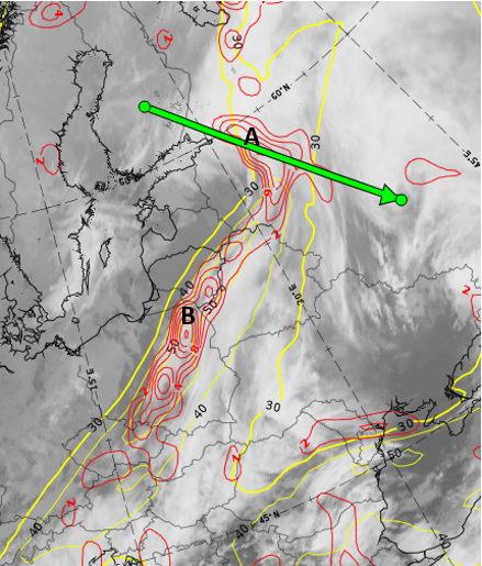
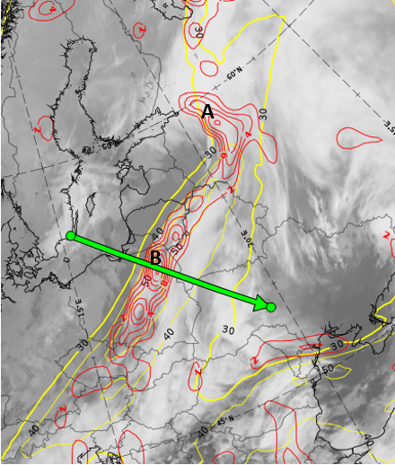 |
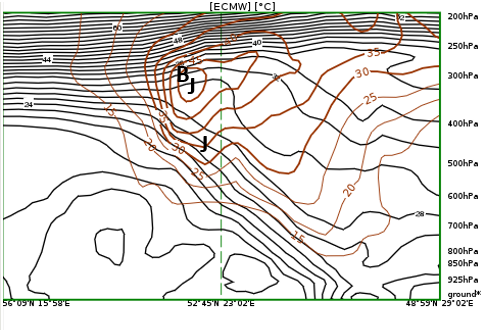
2 February 2018, 18 UTC: The VCS line crosses the jet streak in area B with very high values of CVA. |
Figure 12
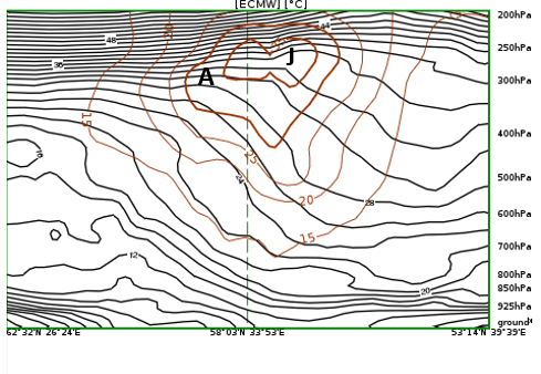
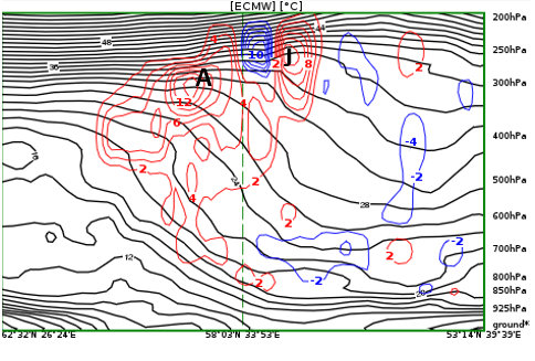
 |
 |
|
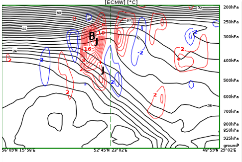
2 February 2018, 18 UTC; VCS line across B Black: (moist) isentropes. |
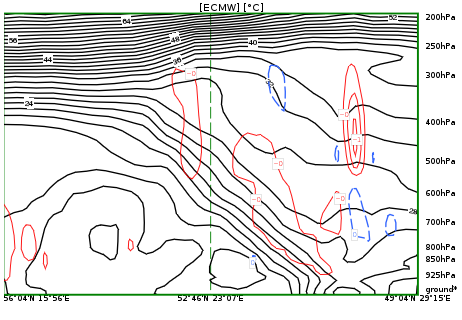 |
Figure 13a-13c
The very distinct CVA maxima accompany the jet core between approximately 500 and 250 hPa, indicating the high vorticity gradient there. It is the result of mathematical computation for a physical environment with frontal upgliding on top of the frontal surface and sinking dry air below it. Some frontal upgliding can be seen on top of the frontal surface, but there is no intensification in the area of the CVA maxima.
 |
2 February 2018, 18 UTC: The VCS crosses the jet streak in area A - which has cloud intensification with high values of CVA - in the left exit region and through the center of the jet streak. |
Figure 14
 |
 |
|
2 February 2018, 18 UTC: VCS line across A Black: (moist) isentropes. |
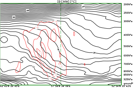 |
Figure 15a-15c
Like in the previous VCS there are CVA maxima accompanying the center of the jet streak (J), but there is an extended CVA maximum (A) away from the axis in the left exit region. It is accompanied by intensified upward motion in a thick layer on top of the frontal surface.
These key parameters and their configuration on isobaric and isentropic surfaces are important features of the CM "Front intensification by jet crossing" and the enhanced cloudiness therein.