Categorical events are not limited to dichotomous (binary, two-category) events and the associated 2*2 contingency tables. A weather element or a variable can be defined in several mutually exhaustive categories like cloudiness or precipitation amount in "k" categories (where k is greater than 2), or rain type categorized into rain - snow - freezing rain, likewise for wind speeds classified into strong gale - gale - no gale (where k=3).

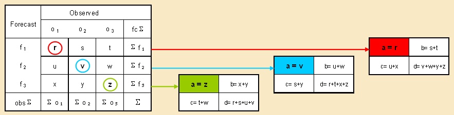
As in the case of binary events, one should initiate the verification effort by compiling a contingency table where the frequencies of forecasts and observations are binned in relevant cells as illustrated in the table below for a 3*3 category case (left-hand-side). A perfect forecasting system would, obviously, have all of the entries along the diagonal (r-v-z) with all of the other bins being =0.

From the contingency table scores presented in the earlier learning units of study in this section only the Proportion Correct (PC) can be directly generalized in situations with more than two categories. The other measures are valid only in the binary "yes/no" forecast situation. To be able to apply the same scores here, one must convert the "k*k" contingency table into a series of 2*2 tables. Each of these is built by considering the "forecast event" distinct from the complementary "non-forecast event", which is, consequently, composed as the union of the remaining "k-1" events. This is showcased on the right-hand-side of the attached table where the same notation is used as on the left-hand-side. The off-diagonal bins provide information on the nature of the forecast errors. Biases (B), for example, exhibit under- or over-prediction of some of the categories, while PODs quantify the forecasting system’s capability of detecting the distinct categorical events.

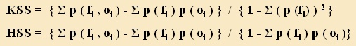
The KSS and HSS skill scores can be generalized for multi-category cases in the form:

where the subscript "i" defines the dimension of the table, p(f _i ,o _i ) represents the joint distribution of forecasts and observations (i.e. the diagonal sum count divided by the total sample size, PC), and p(f _i ) and p(o _i ) are the marginal probability distributions of the forecasts and observations (i.e. row and column sums divided by the total sum), respectively. Both KSS and HSS are measures of the potential improvement in the number of correct forecasts over random ones. The estimation of randomness (expressed by the denominator) is the only difference between these two scores. For a dichotomous case the equations reduce to the corresponding formulae presented in the earlier units of study.