What is a contingency table?

A contingency table is essentially a display format used to analyse and record the relationship between two or more categorical variables. It is the categorical equivalent of the scatterplot used to analyse the relationship between two continuous variables. As always, since we are dealing with verification in this module, the variables to be compared are the forecast and the observation of a weather forecast element, both of which are categorical. The term contingency table was first used by the statistician Karl Pearson in 1904. Contingency tables will normally have as many rows as there are categories in the forecast. For verification purposes, the definition of the forecast and observation variable must be consistent, so a contingency table will have an equal number of rows and columns.

Since dichotomous (two-category) variables are of special interest in meteorology, the emphasis in this module is on the verification methods for the 2*2 contingency tables used to summarize verification datasets for dichotomous variables. Extensions to verification of variables with three or more categories are discussed in the last unit of the module.

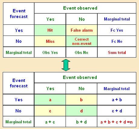
A categorical forecast is a forecast of the occurrence or non-occurrence of a specific event, which must be clearly defined. For example, we may be interested in predicting whether or not the temperature will go below freezing at a particular place. Following the forecast of below freezing (yes) or not below freezing (no), the event will actually occur or not. This leads to four possibilities as laid out in the table shown below. The values of the table are obtained by tallying up the number of times each of the four possible combinations of forecast and observed category occurred:

a = number of times a "yes" forecast was followed by a "yes" occurrence = "hits"
b = number of times a "yes" forecast was followed by a "no" occurrence = "false alarms"
c = number of times a "no" forecast was followed by a "yes" occurrence = "misses"
d = number of times a "no" forecast was followed by a "no" occurrence = "correct non-events"

The table is completed by computing the marginal sums as shown. The value in the lower right hand corner is the total verification sample size and should equal the sum of the four boxes within the table.

Contingency tables are often used to verify forecasts of the occurrence of frost as mentioned above. Other common uses are for the occurrence of precipitation, strong winds (gale force for example) or fog. They are also often used to verify the performance of the forecast for extreme events, for example by setting a threshold precipitation amount or windspeed to separate "extreme" from "non-extreme".

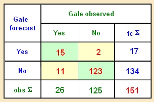
The following exercise will help check your understanding of the entries on a contingency table. This table was used for the verification of gale forecasts.